3. Blade Optimization Example
This example walks through a blade optimization problem with increasing complexity.
All of the iterations use the same geometry input file, BAR-USC.yaml, which describes a baseline design from the NREL-Sandia Big Adaptive Rotor (BAR) project described in this GitHub [repository](https://github.com/NREL/BAR_Designs).
This blade uses carbon fiber-reinforced polymer in the spar cap design. The same modeling_options.yaml file is also common to all iterations and shows that all WISDEM modules are called. The file has dozens of optional inputs hidden. The full list of inputs is available among the `modeling-options`_.
The example file runs four cases one after the other for testing purposes. To run the cases one by one, make sure to comment out all cases at lines 15-18 except the case that should run.
Baseline Design
Whenever conducting a design optimization, it is helpful to first run the starting point design and evaluate the baseline performance. The file, analysis_options_no_opt.yaml, does not have any optimization variables activated and is meant for this purpose. Outputs are generated in the outputs directory.
$ wisdem BAR-USC.yaml modeling_options.yaml analysis_options_no_opt.yaml
Simple Aerodynamic Optimization
The file, analysis_options_aero.yaml, is used to run a blade twist optimization. This is activated by turning on the appropriate design variable flags in the file,
First, we must increase the number of the twist spline control points to 8. We also need to adjust the indices controlling which of these control points can be varied by the optimizer, and which are instead locked. In the twist section, let’s set index_start to 2 (this means that the first 2 of 8 spanwise control points sections are locked), whereas we let all other 6 spanwise control points in the hands of the optimizer. We do this by setting index_end to 8. No need to adjust the maximum decrease and increase that the optimizer can apply to the twist in radians, nor to activate the inverse flag.
For chord, we leave the flag to False.
AEP is the quantity that we maximize,
merit_figure: AEP
To better guide the optimization, we activate a stall margin constraint using the same flag type of setting, with a value of \(5^{\circ} deg \approx 0.087 rad\). If we were to optimize chord, we might also like to constrain chord to a maximum and set a constrain guiding the diameter of the blade root bolt circle.
The maximum iteration limit currently used in the file is 2, to keep the examples short. However, if you want to see more progress in the optimization, change the following lines from:
    optimization:
        flag: True         # Flag to enable optimization
        tol: 1.e-3          # Optimality tolerance
        # max_major_iter: 10  # Maximum number of major design iterations (SNOPT)
        # max_minor_iter: 100 # Maximum number of minor design iterations (SNOPT)
        max_iter: 1         # Maximum number of iterations (SLSQP)
        solver: SLSQP       # Optimization solver. Other options are 'SLSQP' - 'CONMIN'
        step_size: 1.e-3    # Step size for finite differencing
to:
tol: 1.e-3            # Optimality tolerance
max_iter: 10          # Maximum number of minor design iterations
solver: SLSQP         # Optimization solver. Other options are 'SLSQP' - 'CONMIN'
step_size: 1.e-3      # Step size for finite differencing
Now to run the optimization we do,
$ wisdem BAR-USC.yaml modeling_options.yaml analysis_options_aero.yaml
or we comment out lines 16, 17, and 18 in blade_driver.py and we do:
$ python blade_driver.py
or to run in parallel using multiple CPU cores (Mac or Linux only):
$ mpirun -np 4 python blade_driver.py
where the blade_driver.py script is:
import os

from wisdem import run_wisdem
from wisdem.commonse.mpi_tools import MPI
from wisdem.postprocessing.compare_designs import run

mydir = os.path.dirname(os.path.realpath(__file__))  # get path to this file
fname_wt_input = mydir + os.sep + "BAR_USC.yaml"
fname_modeling_options = mydir + os.sep + "modeling_options.yaml"
fname_analysis_options_no_opt = mydir + os.sep + "analysis_options_no_opt.yaml"
fname_analysis_options_aero = mydir + os.sep + "analysis_options_aero.yaml"
fname_analysis_options_struct = mydir + os.sep + "analysis_options_struct.yaml"
fname_analysis_options_aerostruct = mydir + os.sep + "analysis_options_aerostruct.yaml"

wt_opt, modeling_options, analysis_options = run_wisdem(
    fname_wt_input, fname_modeling_options, fname_analysis_options_no_opt
)
wt_opt, modeling_options, analysis_options = run_wisdem(
    fname_wt_input, fname_modeling_options, fname_analysis_options_aero
)
wt_opt, modeling_options, analysis_options = run_wisdem(
    fname_wt_input, fname_modeling_options, fname_analysis_options_struct
)
wt_opt, modeling_options, analysis_options = run_wisdem(
    fname_wt_input, fname_modeling_options, fname_analysis_options_aerostruct
)

if MPI:
    rank = MPI.COMM_WORLD.Get_rank()
else:
    rank = 0

if rank == 0:
    print(
        "RUN COMPLETED. RESULTS ARE AVAILABLE HERE: "
        + os.path.join(mydir, analysis_options["general"]["folder_output"])
    )
The CPU run time is approximately 5 minutes. As the script runs, you will see some output to your terminal, such as performance metrics and some analysis warnings. The optimizer might report that it has failed, but we have artificially limited the number of steps it can take during optimization, so that is expected. Once the optimization terminates, type in the terminal:
$ compare_designs BAR_USC.yaml outputs_aero/blade_out.yaml --labels Init Opt
This script compares the initial and optimized designs.
Some screen output is generated, as well as plots (contained in the outputs folder), such as in Fig. 1 and fig_opt1_twist_opt.
The twist optimization did not have to satisfy a previous constrain for low induction rotors, and after 10 design iterations
AEP grows from 24.34872 to 24.64157 GW*h.
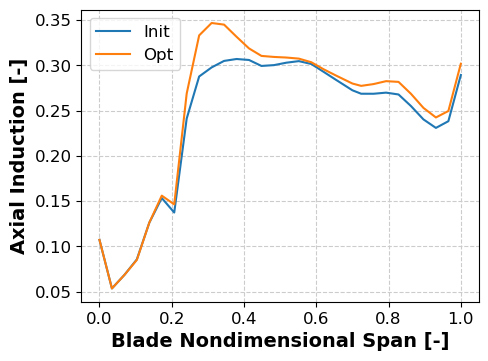
Fig. 1 Initial versus optimized induction profiles
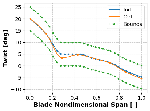
Fig. 2 Initial versus optimized twist profiles
Simple Structural Optimization
Next, we shift from an aerodynamic optimization of the blade to a structural optimization. In this case, we make the following changes,
The design variables as the thickness of the blade structural layers
Spar_cap_ssandSpar_cap_psThe thickness is parameterized in 8 locations along span and can vary between 70 and 130% of the initial value (using the
max_decreaseandmax_increaseoptions)The merit figure is blade mass instead of AEP
A max allowable strain of \(3500 \mu\epsilon\) and the blade tip deflection constrain the problem, but the latter ratio is relaxed to 1.134
To run this optimization problem, we can use the same geometry and modeling input files, and the optimization problem is captured in analysis_options_struct.yaml. The design variables are,
Just increase n_opt to 8 and index_end for both suction- and pressure-side spar caps. The objective function is set to:
merit_figure: blade_mass
and the constraints are,
To run the optimization, just be sure to increase max_iter to 10 and pass in this new analysis options,
$ wisdem BAR-USC.yaml modeling_options.yaml analysis_options_struct.yaml
or, to use the Python driver, be sure to comment out lines 15, 16, and 18 and only leave this uncommented
wt_opt, modeling_options, analysis_options = run_wisdem(fname_wt_input, fname_modeling_options, fname_analysis_options_struct)
and then do,
$ python blade_driver.py
(parallel calculation is also available if desired).
Once the optimization terminates, the same compare_designs script can be used again to plot the differences:
$ compare_designs BAR-USC.yaml outputs_struct/blade_out.yaml --labels Init Opt
The relaxed tip deflection constraint compared to when the baseline was created allows the spar cap thickness to come down and the overall blade mass drops from 51 metric tons to 50 metric tons. This is shown in Fig. 3 and Fig. 4.
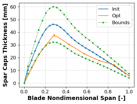
Fig. 3 Baseline versus optimized spar cap thickness profiles
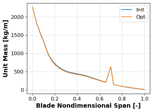
Fig. 4 Baseline versus optimized blade mass profiles. The bump at 70% span corresponds to the spanwise joint of BAR-USC.
WISDEM also estimates the final blade cost, which is reported in the output file outputs_struct/blade_out.csv in the field tcc.blade_cost.
The blade cost after the optimization is USD 538.5k. The initial cost was USD 556.7k. The reduction is larger than blade mass because spar caps are made of expensive carbon fiber.
Aero-Structural Optimization
Finally, we will combine the previous two scenarios and use the levelized cost of energy, LCOE, as a way to balance the power production and minimum mass/cost objectives. This problem formulation is represented in the file, analysis_options_aerostruct.yaml. The design variables are,
    rotor_diameter:
        flag: True
        minimum: 190
        maximum: 240
    blade:
        aero_shape:
            twist:
                flag: True             # Flag to optimize the twist
                inverse: False         # Flag to determine twist from the user-defined desired margin to stall (defined in constraints)
                n_opt: 4               # Number of control points along blade span
                max_decrease: 0.08722222222222221 # Maximum decrease for the twist in [rad] at the n_opt locations
                max_increase: 0.08722222222222221 # Maximum increase for the twist in [rad] at the n_opt locations
                index_start: 2         # Lock the first two DVs from blade root
                index_end: 4           # All DVs close to blade tip are active
            chord:
                flag: True             # Flag to optimize the chord
                n_opt: 4               # Number of control points along blade span
                max_decrease: 0.3      # Minimum multiplicative gain on existing chord at the n_opt locations
                max_increase: 3.       # Maximum multiplicative gain on existing chord at the n_opt locations
                index_start: 2         # Lock the first two DVs from blade root
                index_end: 4           # All DVs close to blade tip are active
        structure:
            spar_cap_ss:
                flag: True             # Flag to optimize the spar cap thickness on the suction side
                n_opt: 4               # Number of control points along blade span
                max_decrease: 0.7      # Maximum nondimensional decrease at the n_opt locations
                max_increase: 1.3      # Maximum nondimensional increase at the n_opt locations
                index_start: 1         # Lock the first DV from blade root
                index_end: 3           # The last DV at blade tip is locked
            spar_cap_ps:
                flag: True             # Flag to optimize the spar cap thickness on the pressure side
                equal_to_suction: True # Flag to impose the spar cap thickness on pressure and suction sides equal
                n_opt: 4               # Number of control points along blade span
                max_decrease: 0.7      # Maximum nondimensional decrease at the n_opt locations
                max_increase: 1.3      # Maximum nondimensional increase at the n_opt locations
                index_start: 1         # Lock the first DV from blade root
                index_end: 3           # The last DV at blade tip is locked
with rotor diameter, blade chord and twist, and spar caps thickness activated as a design variable.
Again, increase the field n_opt to 8 for chord, twist, and spar caps thickness. Also, set index_end to 8 for twist (optimize twist all the way to the tip) and to 7 for chord and spar caps (lock the point at the tip). Do not forget to set index_end to 7 also in the strain constraints.
The objective function set to:
merit_figure: LCOE
and the constraints are,
    blade:
        strains_spar_cap_ss:
            flag: True         # Flag to impose constraints on maximum strains (absolute value) in the spar cap on the blade suction side
            max:    3500.e-6   # Value of maximum strains [-]
            index_start: 1     # Do not enforce constraint at the first station from blade root of the n_opt from spar_cap_ss
            index_end: 3       # Do not enforce constraint at the last station at blade tip of the n_opt from spar_cap_ss
        strains_spar_cap_ps:
            flag: True         # Flag to impose constraints on maximum strains (absolute value) in the spar cap on the blade pressure side
            max:    3500.e-6   # Value of maximum strains [-]
            index_start: 1     # Do not enforce constraint at the first station from blade root of the n_opt from spar_cap_ps
            index_end: 3       # Do not enforce constraint at the last station at blade tip of the n_opt from spar_cap_ps
        strains_te_ss:
            flag: False        # Flag to impose constraints on maximum strains (absolute value) in the spar cap on the blade suction side
            max:    3500.e-6   # Value of maximum strains [-]
            index_start: 1     # Do not enforce constraint at the first station from blade root of the n_opt from spar_cap_ss
            index_end: 3       # Do not enforce constraint at the last station at blade tip of the n_opt from spar_cap_ss
        strains_te_ps:
            flag: False        # Flag to impose constraints on maximum strains (absolute value) in the spar cap on the blade pressure side
            max:    3500.e-6   # Value of maximum strains [-]
            index_start: 1     # Do not enforce constraint at the first station from blade root of the n_opt from spar_cap_ps
            index_end: 3       # Do not enforce constraint at the last station at blade tip of the n_opt from spar_cap_ps
        tip_deflection:
            flag: True
            margin: 1.4175
        stall:
            flag: True    # Constraint on minimum stall margin
            margin: 0.087 # Value of minimum stall margin in [rad]
One more change for this final example is tighter optimization convergence tolerance (\(1e-5\)), because LCOE tends to move only a very small amount from one design to the next,
    optimization:
        flag: True         # Flag to enable optimization
        tol: 1.e-5          # Optimality tolerance
        # max_major_iter: 10  # Maximum number of major design iterations (SNOPT)
        # max_minor_iter: 100 # Maximum number of minor design iterations (SNOPT)
        max_iter: 1         # Maximum number of iterations (SLSQP)
        solver: SLSQP       # Optimization solver. Other options are 'SLSQP' - 'CONMIN'
        step_size: 1.e-3    # Step size for finite differencing
To run the optimization, just be sure to pass in this new analysis options
$ wisdem BAR-USC.yaml modeling_options.yaml analysis_options_aerostruct.yaml
or, to use the Python driver, be sure run line 18 as above to be
wt_opt, modeling_options, analysis_options = run_wisdem(fname_wt_input, fname_modeling_options, fname_analysis_options_aerostruct)
and then do,
$ python blade_driver.py
We can then use the compare_designs command in the same way as above to plot the optimization results, two of which are shown in, fig_opt3_induction and Fig. 6. With more moving parts, it can be harder to interpret the results. In the end, LCOE is increased marginally because the initial blade tip deflection constraint, which is set to 1.4175 in the analysis options yaml, is initially violated and the optimizer has to stiffen up and shorten the blade. The rotor diameter is reduced from 206 m to 202.7 and twist is simultaneously adjusted to keep performance up.
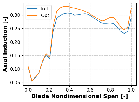
Fig. 5 Baseline versus optimized induction profiles
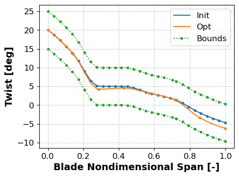
Fig. 6 Baseline versus optimized twist profiles