10. CCBlade Examples

Three examples are shown below. The first is a complete setup for the NREL 5-MW model, the second shows how to model blade precurvature, and the final shows how to get the provided analytic gradients. Each complete example is also included within the WISDEM/examples/10_ccblade directory.

NREL 5-MW

One example of a CCBlade application is the simulation of the NREL 5-MW reference model’s aerodynamic performance. First, define the geometry and atmospheric properties.

from math import pi

import numpy as np
import matplotlib.pyplot as plt

from wisdem.ccblade.ccblade import CCBlade, CCAirfoil

plot_flag = False

# geometry
Rhub = 1.5
Rtip = 63.0

r = np.array(
    [
        2.8667,
        5.6000,
        8.3333,
        11.7500,
        15.8500,
        19.9500,
        24.0500,
        28.1500,
        32.2500,
        36.3500,
        40.4500,
        44.5500,
        48.6500,
        52.7500,
        56.1667,
        58.9000,
        61.6333,
    ]
)
chord = np.array(
    [
        3.542,
        3.854,
        4.167,
        4.557,
        4.652,
        4.458,
        4.249,
        4.007,
        3.748,
        3.502,
        3.256,
        3.010,
        2.764,
        2.518,
        2.313,
        2.086,
        1.419,
    ]
)
theta = np.array(
    [
        13.308,
        13.308,
        13.308,
        13.308,
        11.480,
        10.162,
        9.011,
        7.795,
        6.544,
        5.361,
        4.188,
        3.125,
        2.319,
        1.526,
        0.863,
        0.370,
        0.106,
    ]
)
B = 3  # number of blades

tilt = 5.0
precone = 2.5
yaw = 0.0

nSector = 8  # azimuthal discretization

# atmosphere
rho = 1.225
mu = 1.81206e-5

# power-law wind shear profile
shearExp = 0.2
hubHt = 90.0

Airfoil aerodynamic data is specified using the CCAirfoil class. Rather than use the default constructor, this example uses the special constructor designed to read AeroDyn files directly CCAirfoil.initFromAerodynFile().

import os
from wisdem.inputs.validation import load_geometry_yaml
baseyaml = os.path.join(os.path.dirname(os.path.dirname(os.path.realpath(__file__))), "02_reference_turbines", "nrel5mw.yaml")
data = load_geometry_yaml(baseyaml)
af = data['airfoils']
af_names = ["Cylinder", "Cylinder", "DU40_A17", "DU35_A17", "DU30_A17", "DU25_A17", "DU21_A17", "NACA64_A17"]
airfoil_types = [0] * len(af_names)
for i in range(len(af_names)):
    for j in range(len(af)):
        if af[j]["name"] == af_names[i]:
            polars = af[j]['polars'][0]
            airfoil_types[i] = CCAirfoil(
                np.rad2deg(polars["c_l"]["grid"]),
                [polars["re"]],
                polars["c_l"]["values"],
                polars["c_d"]["values"],
                polars["c_m"]["values"],
            )

# place at appropriate radial stations
af_idx = [0, 0, 1, 2, 3, 3, 4, 5, 5, 6, 6, 7, 7, 7, 7, 7, 7]

af = [0] * len(r)
for i in range(len(r)):
    af[i] = airfoil_types[af_idx[i]]

Next, construct the CCBlade object.

# create CCBlade object
rotor = CCBlade(r, chord, theta, af, Rhub, Rtip, B, rho, mu, precone, tilt, yaw, shearExp, hubHt, nSector)

Evaluate the distributed loads at a chosen set of operating conditions.

# set conditions
Uinf = 10.0
tsr = 7.55
pitch = 0.0
Omega = Uinf * tsr / Rtip * 30.0 / pi  # convert to RPM
azimuth = 0.0

# evaluate distributed loads
loads, derivs = rotor.distributedAeroLoads(Uinf, Omega, pitch, azimuth)
Np = loads["Np"]
Tp = loads["Tp"]

Plot the flapwise and lead-lag aerodynamic loading

# plot
rstar = (r - Rhub) / (Rtip - Rhub)

# append zero at root and tip
rstar = np.concatenate([[0.0], rstar, [1.0]])
Np = np.concatenate([[0.0], Np, [0.0]])
Tp = np.concatenate([[0.0], Tp, [0.0]])

if plot_flag:
    plt.plot(rstar, Tp / 1e3, label="lead-lag")
    plt.plot(rstar, Np / 1e3, label="flapwise")
    plt.xlabel("blade fraction")
    plt.ylabel("distributed aerodynamic loads (kN)")
    plt.legend(loc="upper left")
    plt.grid()
    plt.show()

as shown in Figure 16.

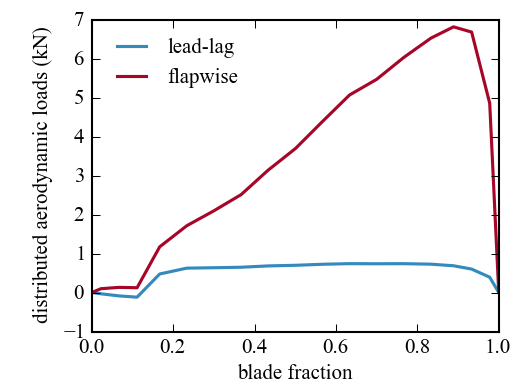
Fig. 16 Flapwise and lead-lag aerodynamic loads along blade.

To get the power, thrust, and torque at the same conditions (in both absolute and coefficient form), use the evaluate method. This is generally used for generating power curves so it expects array_like input. For this example a list of size one is used.

outputs, derivs = rotor.evaluate([Uinf], [Omega], [pitch])

P = outputs["P"]
T = outputs["T"]
Q = outputs["Q"]

outputs, derivs = rotor.evaluate([Uinf], [Omega], [pitch], coefficients=True)

CP = outputs["CP"]
CT = outputs["CT"]
CQ = outputs["CQ"]

print("CP =", CP)
print("CT =", CT)
print("CQ =", CQ)

The result is

>>> CP = [ 0.46488096]
>>> CT = [ 0.76926398]
>>> CQ = [ 0.0616323]

Note that the outputs are Numpy arrays (of length 1 for this example). To generate a nondimensional power curve (\(\lambda\) vs \(c_p\)):

# velocity has a small amount of Reynolds number dependence
tsr = np.linspace(2, 14, 50)
Omega = 10.0 * np.ones_like(tsr)
Uinf = Omega * pi / 30.0 * Rtip / tsr
pitch = np.zeros_like(tsr)

outputs, derivs = rotor.evaluate(Uinf, Omega, pitch, coefficients=True)

CP = outputs["CP"]
CT = outputs["CT"]
CQ = outputs["CQ"]

if plot_flag:
    plt.figure()
    plt.plot(tsr, CP)
    plt.xlabel("$\lambda$")
    plt.ylabel("$c_p$")
    plt.show()

Figure 17 shows the resulting plot.

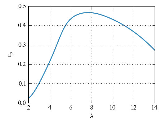
Fig. 17 Power coefficient as a function of tip-speed ratio.

CCBlade provides a few additional options in its constructor. The other options are shown in the following example with their default values.

# create CCBlade object
rotor = CCBlade(r, chord, theta, af, Rhub, Rtip, B, rho, mu,
                precone, tilt, yaw, shearExp, hubHt, nSector
                tiploss=True, hubloss=True, wakerotation=True, usecd=True, iterRe=1)

The parameters tiploss and hubloss toggle Prandtl tip and hub losses respectively. The parameter wakerotation toggles wake swirl (i.e., \(a^\prime = 0\)). The parameter usecd can be used to disable the inclusion of drag in the calculation of the induction factors (it is always used in calculations of the distributed loads). However, doing so may cause potential failure in the solution methodology (see [Nin13]). In practice, it should work fine, but special care for that particular case has not yet been examined, and the default implementation allows for the possibility of convergence failure. All four of these parameters are True by default. The parameter iterRe is for advanced usage. Referring to [Nin13], this parameter controls the number of internal iterations on the Reynolds number. One iteration is almost always sufficient, but for high accuracy in the Reynolds number iterRe could be set at 2. Anything larger than that is unnecessary.

Precurve

CCBlade can also simulate blades with precurve. This is done by using the precurve and precurveTip parameters. These correspond precisely to the r and Rtip parameters. Precurve is defined as the position of the blade reference axis in the x-direction of the blade-aligned coordinate system (r is the position in the z-direction of the same coordinate system). Presweep can be specified in the same manner, by using the presweep and presweepTip parameters (position in blade-aligned y-axis). Generally, it is advisable to set precone=0 for blades with precurve. There is no loss of generality in defining the blade shape, and including a nonzero precone would change the rotor diameter in a nonlinear way. As an example, a downwind machine with significant curvature could be simulated using:

precone = 0.0
precurve = np.linspace(0, 4.9, len(r)) ** 2
precurveTip = 25.0


# create CCBlade object
rotor = CCBlade(
    r,
    chord,
    theta,
    af,
    Rhub,
    Rtip,
    B,
    rho,
    mu,
    precone,
    tilt,
    yaw,
    shearExp,
    hubHt,
    nSector,
    precurve=precurve,
    precurveTip=precurveTip,
)

The shape of the blade is seen in Figure 18. Note that the radius of the blade is preserved because we have set the precone angle to zero.

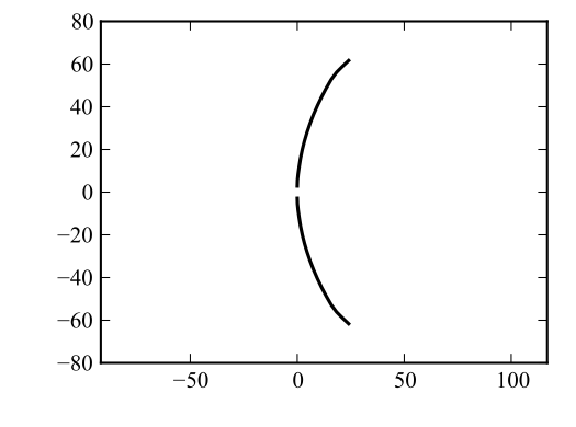
Fig. 18 Profile of an example (highly) precurved blade.

Gradients

CCBlade optionally provides analytic gradients of every output with respect to all design variables. This is accomplished using an adjoint method (direct method is identical because there is only one state variable at each blade section). Partial derivatives are provided by Tapenade and hand calculations. Starting with the previous example for the NREL 5-MW reference model we add the keyword value derivatives=True in the constructor.

# create CCBlade object
rotor = CCBlade(
    r, chord, theta, af, Rhub, Rtip, B, rho, mu, precone, tilt, yaw, shearExp, hubHt, nSector, derivatives=True
)

Now when we ask for the distributed loads, we also get the gradients. The gradients are returned as a dictionary containing 2D arrays. These can be accessed as follows:

loads, derivs = rotor.distributedAeroLoads(Uinf, Omega, pitch, azimuth)
Np = loads["Np"]
Tp = loads["Tp"]
dNp = derivs["dNp"]
dTp = derivs["dTp"]

n = len(r)

# n x n (diagonal)
dNp_dr = dNp["dr"]
dNp_dchord = dNp["dchord"]
dNp_dtheta = dNp["dtheta"]
dNp_dpresweep = dNp["dpresweep"]

# n x n (tridiagonal)
dNp_dprecurve = dNp["dprecurve"]

# n x 1
dNp_dRhub = dNp["dRhub"]
dNp_dRtip = dNp["dRtip"]
dNp_dprecone = dNp["dprecone"]
dNp_dtilt = dNp["dtilt"]
dNp_dhubHt = dNp["dhubHt"]
dNp_dyaw = dNp["dyaw"]
dNp_dazimuth = dNp["dazimuth"]
dNp_dUinf = dNp["dUinf"]
dNp_dOmega = dNp["dOmega"]
dNp_dpitch = dNp["dpitch"]

Even though many of the matrices are diagonal, the full Jacobian is returned for consistency. We can compare against finite differencing as follows (with a randomly chosen station along the blade):

idx = 8
delta = 1e-6 * r[idx]
r[idx] += delta

rotor_fd = CCBlade(
    r, chord, theta, af, Rhub, Rtip, B, rho, mu, precone, tilt, yaw, shearExp, hubHt, nSector, derivatives=False
)

r[idx] -= delta

loads, derivs = rotor_fd.distributedAeroLoads(Uinf, Omega, pitch, azimuth)
Npd = loads["Np"]
Tpd = loads["Tp"]

dNp_dr_fd = (Npd - Np) / delta
dTp_dr_fd = (Tpd - Tp) / delta

print("(analytic) dNp_i/dr_i =", dNp_dr[idx, idx])
print("(fin diff) dNp_i/dr_i =", dNp_dr_fd[idx])
print()

The output is:

>>> (analytic) dNp_i/dr_i = 107.680395098
>>> (fin diff) dNp_i/dr_i = 107.680370762

Similarly, when we compute thrust, torque, and power we also get the gradients (for either the non-dimensional or dimensional form). The gradients are also returned as a dictionary containing 2D Jacobians.

loads, derivs = rotor.evaluate([Uinf], [Omega], [pitch])
P = loads["P"]
T = loads["T"]
Q = loads["Q"]

dP = derivs["dP"]
dT = derivs["dT"]
dQ = derivs["dQ"]

npts = len(P)

# npts x 1
dP_dprecone = dP["dprecone"]
dP_dtilt = dP["dtilt"]
dP_dhubHt = dP["dhubHt"]
dP_dRhub = dP["dRhub"]
dP_dRtip = dP["dRtip"]
dP_dprecurveTip = dP["dprecurveTip"]
dP_dpresweepTip = dP["dpresweepTip"]
dP_dyaw = dP["dyaw"]

# npts x npts
dP_dUinf = dP["dUinf"]
dP_dOmega = dP["dOmega"]
dP_dpitch = dP["dpitch"]

# npts x n
dP_dr = dP["dr"]
dP_dchord = dP["dchord"]
dP_dtheta = dP["dtheta"]
dP_dprecurve = dP["dprecurve"]
dP_dpresweep = dP["dpresweep"]

Let us compare the derivative of power against finite differencing for one of the scalar quantities (precone):

delta = 1e-6 * precone
precone += delta

rotor_fd = CCBlade(
    r, chord, theta, af, Rhub, Rtip, B, rho, mu, precone, tilt, yaw, shearExp, hubHt, nSector, derivatives=False
)

precone -= delta

loads, derivs = rotor_fd.evaluate([Uinf], [Omega], [pitch], coefficients=False)
Pd = loads["P"]
Td = loads["T"]
Qd = loads["Q"]

dT_dprecone_fd = (Td - T) / delta
dQ_dprecone_fd = (Qd - Q) / delta
dP_dprecone_fd = (Pd - P) / delta

print("(analytic) dP/dprecone =", dP_dprecone[0, 0])
print("(fin diff) dP/dprecone =", dP_dprecone_fd[0])
print()

>>> (analytic) dP/dprecone = -4585.70729746
>>> (fin diff) dP/dprecone = -4585.71072668

Finally, we compare the derivative of power against finite differencing for one of the vector quantities (r) at a random index:

idx = 12
delta = 1e-6 * r[idx]
r[idx] += delta

rotor_fd = CCBlade(
    r, chord, theta, af, Rhub, Rtip, B, rho, mu, precone, tilt, yaw, shearExp, hubHt, nSector, derivatives=False
)

r[idx] -= delta

loads, derivs = rotor_fd.evaluate([Uinf], [Omega], [pitch], coefficients=False)
Pd = loads["P"]
Td = loads["T"]
Qd = loads["Q"]

dT_dr_fd = (Td - T) / delta
dQ_dr_fd = (Qd - Q) / delta
dP_dr_fd = (Pd - P) / delta

print("(analytic) dP/dr_i =", dP_dr[0, idx])
print("(fin diff) dP/dr_i =", dP_dr_fd[0])
print()

>>> (analytic) dP/dr_i = 848.368037506
>>> (fin diff) dP/dr_i = 848.355994992

For more comprehensive comparison to finite differencing, see the unit tests contained in wisdem/test/test_ccblade/test_gradients.py.