2. Running the NREL 5-MW and IEA Wind 15-MW Reference Wind Turbines
The next example involves running two reference turbine examples, the NREL 5-MW land-based and IEA Wind 15-MW offshore fixed-bottom turbines. There are multiple ways to run WISDEM, each is perfectly valid and users should adopt whatever approach they are most comfortable with.
Calling WISDEM
Option 1. Use the GUI
Installing WISDEM creates a wisdem command that should be available at the command prompt (a terminal prompt on Linux / Mac machines or the Anaconda PowerShell prompt for Windows). Just typing wisdem at the command line opens the GUI. From there, you can use the dialogue menus to load in the yaml input files and run WISDEM.
Option 2. Pass YAML-files directly to the wisdem command
Installing WISDEM creates a wisdem command that should be available at the command prompt (a terminal prompt on Linux / Mac machines or the Anaconda PowerShell prompt for Windows). You can pass that command the three input yaml-files in order to run WISDEM.
$ wisdem nrel5mw.yaml modeling_options.yaml analysis_options.yaml
Alternatively, you can create a summary WISDEM file that points to each file,
$ wisdem nrel5mw_driver.yaml
Where the contents of nrel5mw_driver.yaml are,
geometry_file: nrel5mw.yaml
modeling_file: modeling_options.yaml
analysis_file: analysis_options.yaml
Note that to run the IEA Wind 15-MW reference wind turbine, simply substitute the file, IEA-15-240-RWT.yaml, in as the geometry file. The modeling_options.yaml and analysis_options.yaml file can remain the same.
Option 3. Call WISDEM from a Python Script
For those users who are comfortable with Python scripting, the WISDEM yaml input files can also be passed as path names to the main WISDEM function in this way,
$ python nrel5mw_driver.py
Where the contents of nrel5mw_driver.py are,
import os

from wisdem import run_wisdem

## File management
mydir = os.path.dirname(os.path.realpath(__file__))  # get path to this file
fname_wt_input = mydir + os.sep + "nrel5mw.yaml"
fname_modeling_options = mydir + os.sep + "modeling_options.yaml"
fname_analysis_options = mydir + os.sep + "analysis_options.yaml"

wt_opt, analysis_options, opt_options = run_wisdem(fname_wt_input, fname_modeling_options, fname_analysis_options)
Screen Output
Successfully running WISDEM should show the following screen output for the NREL 5-MW reference wind turbine:
==
wt
==
NL: NLBGS Converged in 2 iterations
########################################
Objectives
Turbine AEP: 24.0796812417 GWh
Blade Mass:  16403.6823269407 kg
LCOE:        49.4740771484 USD/MWh
Tip Defl.:   4.1950872846 m
########################################
And this output for the IEA Wind 15-MW reference wind turbine:
==
wt
==
WARNING: the blade cost model is used beyond its applicability range. No team can limit the main mold cycle time to 24 hours. 100 workers are assumed at the low-pressure mold, but this is incorrect.
WARNING: the blade cost model is used beyond its applicability range. No team can limit the main mold cycle time to 24 hours. 100 workers are assumed at the high-pressure mold, but this is incorrect.
WARNING: the blade cost model is used beyond its applicability range. No team can limit the assembly cycle time to 24 hours. 100 workers are assumed at the assembly line, but this is incorrect.
|
| ==========
| wt.drivese
| ==========
| NL: NLBGS Converged in 2 iterations
NL: NLBGSSolver 'NL: NLBGS' on system 'wt' failed to converge in 2 iterations.
ORBIT library intialized at '/Users/gbarter/devel/WISDEM/wisdem/library'
########################################
Objectives
Turbine AEP: 78.0794202708 GWh
Blade Mass: 73310.0985877902 kg
LCOE: 71.9371232305 USD/MWh
Tip Defl.: 22.7001875342 m
########################################
Some helpful summary information is printed to the screen. More detailed output can be found in the outputs directory. This creates output files that can be read-in by Matlab, Numpy, Python pickle-package, and Excel. These files have the complete list of all WISDEM variables (with extended naming based on their OpenMDAO Group hierarchy) and the associated values. An output yaml-file is also written, in case any input values were altered in the course of the analysis.
$ ls -1 outputs

refturb_output.mat
refturb_output.npz
refturb_output.pkl
refturb_output.xlsx
refturb_output.yaml
refturb_output-modeling.yaml
refturb_output-analysis.yaml
Extension |
Description |
|---|---|
|
MatLab output format |
|
Archive of NumPy arrays |
|
Python Pickle format |
|
Microsoft Excel format |
|
YAML format |
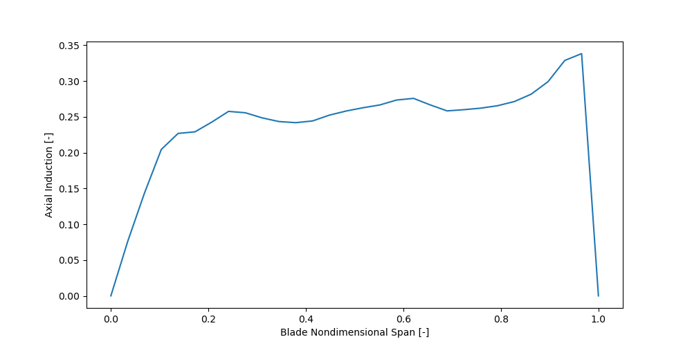
As an example, the sample_plot.py script plots Axial Induction versus Blade Nondimensional Span by extracting the values from the Python pickle file. The script content is:
import matplotlib.pyplot as plt

from wisdem.glue_code.runWISDEM import load_wisdem

refturb, _, _ = load_wisdem("outputs/refturb_output.pkl")
xs = refturb["wt.wt_init.blade.outer_shape_bem.compute_blade_outer_shape_bem.s_default"]
ys = refturb["wt.rp.powercurve.compute_power_curve.ax_induct_regII"]
fig, ax = plt.subplots(nrows=1, ncols=1, figsize=(10, 5))
ax.plot(xs, ys)
ax.set_xlabel("Blade Nondimensional Span [-]")
ax.set_ylabel("Axial Induction [-]")
plt.show()
This script generates the following plot:
