First Steps in WISDEM

WISDEM just needs three input files for many optimization and analysis operations. These files specify the geometry of the turbine, modeling options, and analysis options. The files and details about them are outlined in the following table:

Description	Suggested Default to Modify	Where to learn more
Geometry of the turbine	nrel5mw.yaml	WindIO docs
Modeling options	modeling_options.yaml	Modeling Options Inputs
Analysis options	analysis_options.yaml	Analysis Options Inputs

There are two options to run WISDEM with these files. The first option is to use a text editor to modify files and to run WISDEM from the command line. The second option is to edit the files with a GUI and run WISDEM with the click of a button. This document will describe both of these options in turn.

The first step for either option is to make copies of example files

Before you start editing your WISDEM input files, please make copies of the original files in a separate folder. This ensures that if you edit copies of the original files you can always revert back to a version of the files that is known to execute successfully. Each one of the linked files in the table is a good starting point for a turbine simulation.

Option 1: Text editor and command line

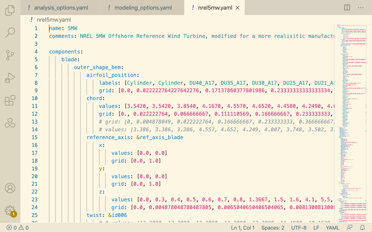
First, edit the files in the text editor. You can use the ontology guide as a reference when you create the geometry file. Edit the geometry, modeling options, and analysis options as you need them:

Second, after you are done editing, run WISDEM from the command line with a command of the following form:

conda activate wisdem-env
wisdem [geometry file].yaml [modeling file].yaml [analysis file].yaml

Substitute [geometry file].yaml with the filename for your geometry, [modeling file].yaml with your modeling filename and [analysis file].yaml with your analysis filename. If you were to run WISDEM with the example files provided above, the command would be wisdem nrel5mw.yaml modeling_options.yaml analysis_options.yaml

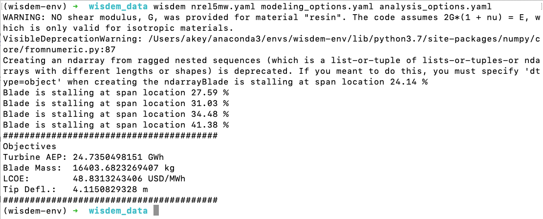
WISDEM will produce output messages as it runs. At the end, if everything executes correctly, you will see output similar to the following:

Objectives
Turbine AEP: 24.7350498151 GWh
Blade Mass:  16403.6823269407 kg
LCOE:        48.8313243406 USD/MWh
Tip Defl.:   4.1150829328 m

A command line session to execute WISDEM in this way will look similar to the following figure. This will vary depending on your installation, but the basic elements should be there. Note the final lines that WISDEM outputs, as shown above:

Outputs from the run are stored in the outputs folder that is created within the folder in which you executed the WISDEM command. These are described in detail in the outputs section of this document.

Option 2: WISDEM GUI

Launching the GUI is simpler than launching the command line. Activate you environment and execute the WISDEM GUI with the following commands:

conda activate wisdem-env
wisdem

The WISDEM GUI is laid out from left to right to edit the geometry, modeling, and analysis files. The upper part of the interface shows a status bar and at the right side there is a Run WISDEM button.

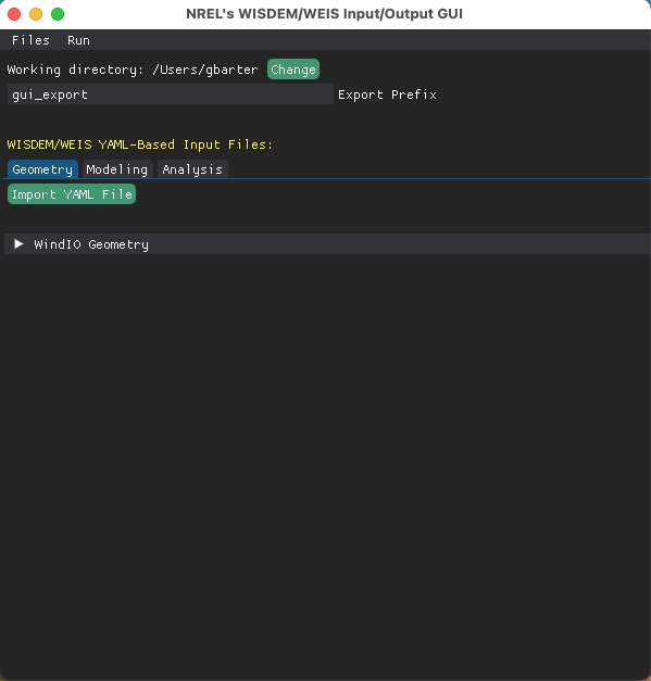
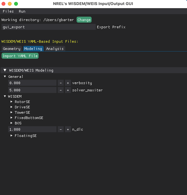
When you start the WISDEM GUI, a window similar to the following will appear (there might be some differences depending on whether you are running Windows or macOS or Linux:

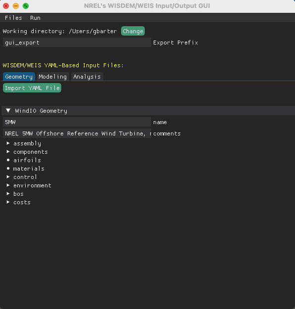
First, load a geometry file. By default, the WindIO description of the IEA Wind 15-MW reference turbine is loaded, but we will load in the NREL 5-MW reference turbine as a demonstration. The nrel5mw.yaml file can be found in the examples directory of WISDEM under the 02_reference_turbines heading. Load this file by clicking the Import YAML File button under the Geometry tab for WISDEM/WEIS YAML-Based Input Files, and selecting your copy of nrel5mw.yaml. If you expand the collapsible tree titled, WindIO Geometry, you can visually descend into the file contents and edit the entries.

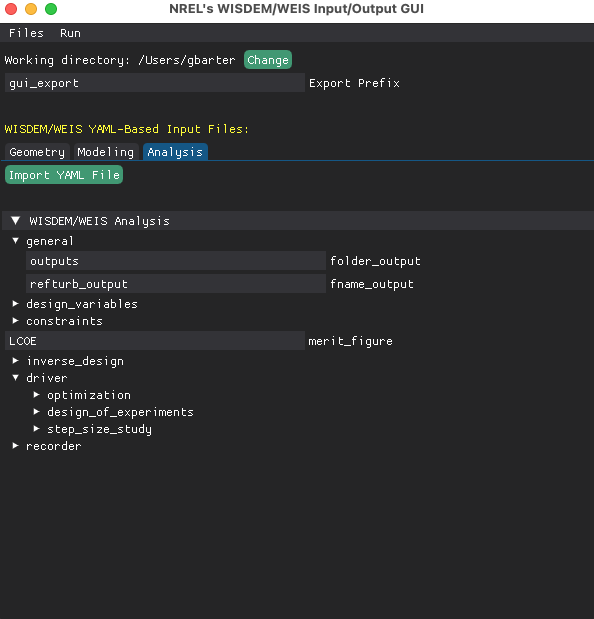
You can similarly load in modeling and analysis yaml-files, with defaults already loaded under the Modeling and Analysis tabs. You can edit the entries if you like:

You are now ready to run WISDEM! In the GUI, click on Run WISDEM/WEIS underneath the Run menu header. The GUI-specified entries will be written to files in the Working directory specified at the top of the GUI using the prefix string next to Export Prefix. You can change these prior to running WISDEM if you like. While running WISDEM in the background, the GUI will be inactive:

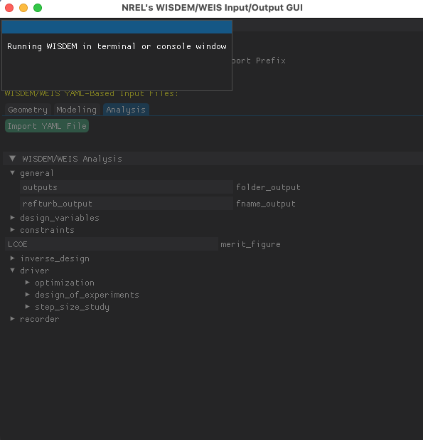
Depending on whether you are running a design optimization or not, WISDEM may take a while to run. The GUI will become active again once the run is complete. Output files can be found in the Working directory.

Working with Outputs Manually

In the outputs folder there are several files. Each of them hold all the output variables from a run but are in different formats for various environments:

$ ls -1 outputs

refturb_output.mat
refturb_output.npz
refturb_output.pkl
refturb_output.xlsx
refturb_output.yaml
refturb_output-modeling.yaml
refturb_output-analysis.yaml

Extension	Description
.mat	MatLab output format
.npz	Archive of NumPy arrays
.pkl	Python Pickle format
.xlsx	Microsoft Excel format
.yaml	YAML format

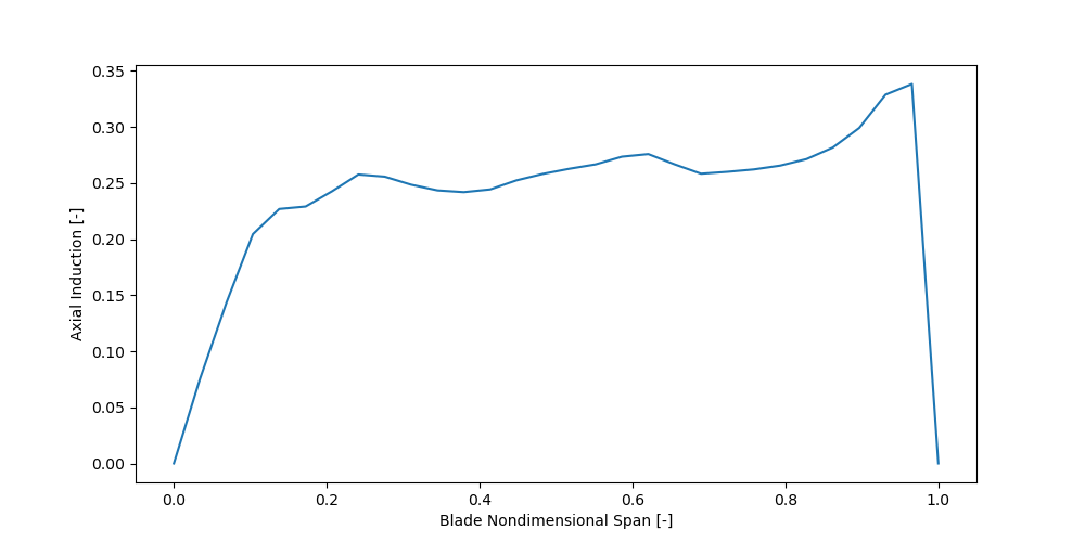
As an example, the sample_plot.py script plots Axial Induction versus Blade Nondimensional Span by extracting the values from the Python pickle file. The script content is:

import matplotlib.pyplot as plt

from wisdem.glue_code.runWISDEM import load_wisdem

refturb, _, _ = load_wisdem("outputs/refturb_output.pkl")
xs = refturb["wt.wt_init.blade.outer_shape_bem.compute_blade_outer_shape_bem.s_default"]
ys = refturb["wt.rp.powercurve.compute_power_curve.ax_induct_regII"]
fig, ax = plt.subplots(nrows=1, ncols=1, figsize=(10, 5))
ax.plot(xs, ys)
ax.set_xlabel("Blade Nondimensional Span [-]")
ax.set_ylabel("Axial Induction [-]")
plt.show()

This script generates the following plot:

Working with Outputs Using compare_designs

WISDEM also comes with a built-in command to help post-process results automatically. Just as there is a wisdem console command installed, there is a compare_designs command that plots and prints WISDEM results given a turbine yaml file. If the turbine yaml file is part of an output series, the values are loaded, otherwise it runs WISDEM using a default set of options. This command can be used within any directory where you have turbine yaml files you want to investigate.

For example, you can use the command to view the results from the previous example simulation. Invoke the command by typing compare_designs outputs/refturb_output.yaml in your terminal. Since this example was just run, it loads in the values, then prints key results to screen and saves plots for variable distributions along the blade span.

You can also compare designs of multiple turbine yaml files using this command, which is especially useful for comparing initial and optimal designs. To do this, simply list as many yaml files as you want to compare after invoking the compare_designs command. Additionally, you can supply your own modeling and analysis options if you want to customize the type of simulation performed when comparing results.

For any further modifications, you can customize the output of the compare_designs command by locally editing the script in the wisdem/postprocessing/compare_designs.py file.