Theory
Design Load Cases (DLCs)
The user must specify the metocean conditions that drive the wind and wave loads upon the floating substructure. FloatingSE currently only uses the single load case of maximum thrust coincident with maximum wave loading to drive the substructure design. The assumption is that this load case would be the driver for substructure sizing and stability. Ideally, multiple DLCs and metocean conditions would be used for design optimization. The capability to optimize over multiple DLCs will be added to future versions of the model. By not currently including a formal set of IEC DLCs, the conceptual designs derived in this work should be considered preliminary and subject to extensive revision once other load cases, and higher-fidelity analysis, is brought to bear.
Load Path
As with other WISDEM models, the primary simplification in FloatingSE is the treatment of all loads as pseudo-static. This approximation significantly reduces computational time and resources, since an accurate calculation of dynamic loads requires more sophisticated numerical tools and simulations. However, dynamic effects can still dominate drive component sizing for floating platforms, thus the static loading assumption gives a rough approximation of the total loading. Furthermore, fatigue effects and structural lifetime estimates are also excluded for now, but could be incorporated in future developments.
A floating wind turbine undergoes loading from a number of sources. The primary loading source for the tower comes from the aerodynamic loads induced by the rotor. The substructure must resist the combination of both rotor loads and hydrodynamics loads, with the latter becoming more and more important as water depth and wave heights increase. FloatingSE, together with other WISDEM modules, accounts for these two dominant load sources, as well as the self-loading of gravity loads. Other sources of loading, such as installation loads, accidental loads, vortex-induced vibrations, ice, and seismic loads are ignored.
Wind and Wave Loads
Wind drag loads are applied to the tower body and the upper part of the substructure that extends above the waterline. They are not applied to connecting truss members that may be part of the substructure geometry. These drag loads are computed assuming the tower and columns are smooth circular cross-sections and that the drag coefficient can be selected as a function of the flow Reynolds number [Ros61]. The aerodynamic drag force is a function of height, since the wind profile and cross-sectional geometry varies along that dimension. For the wind profile, the standard power-law scaling is used,
where \(U_a(z)\) is the wind velocity as a function of height, \(U_{ref}\) is a reference wind speed measured at a reference height, \(z_{ref}\), and \(\alpha\) is the shear exponent used in the power-law approximation of wind profiles. The wind profile then feeds the aerodynamic drag, Reynolds number, and drag coefficient,
where \(Re_d\) is the Reynolds number based on diameter, \(\rho_a\) and \(\mu_a\) are the density and viscosity of air, \(d(z)\) is the diameter of the column as a function of height, \(c_d\) is the 2-D drag coefficient, and \(dF(z)\) is the force per unit length in the z-direction.
Wave drag loads arise from similar processes, but are computed using Morison’s equation, a semi-empirical expression that predicts the total hydrodynamic loads. It is comprised of two components, one for viscous drag contributions and another for inertial effects (which includes incident, diffracted, and radiated wave effects). For flow past structures with circular cross sections, Morison’s equation for force per unit length (\(dF(z)\)) takes the form,
where \(C_m\) is the added mass coefficient (assumed to be \(C_m=2\)), \(U_w(z)\) is the current speed as a function of height, \(\dot{U}_w(z)\) is the acceleration as a function of height, and the Reynolds number is computed by substituting in the appropriate properties for water,
To compute Morison’s equation, expressions for local fluid velocity and acceleration are required. Wave particle velocity (not the same as the bulk velocity of the wave) is assumed to follow linear (Airy) wave theory
where \(\omega\) is the circular frequency, \(T\) is the wave period, \(a\) is the wave amplitude (half of the significant wave height), \(D\) is the total water depth, \(g\) is the acceleration of gravity, and \(\kappa\) is the wave number numerically computed from the dispersion relationship given as the last expression in Equation [eqn:Uwave]. Note that the horizontal particle velocity varies in time and space (by the \(\kappa x - \omega t\)) term. Thus, the individual particles in the wave are also accelerating at different rates,
For simplicity, FloatingSE only considers the maximum velocity and acceleration at a given height, and makes a conservative assumption that they are concurrent in time and space. This essentially means ignoring the \(\kappa x - \omega t\) term, since the maximum of any hyperbolic sine or cosine term is one.
Rotor Nacelle Assembly (RNA) Loads
From a quasi-steady-state point of view, the RNA loads reduce to three forces and three moments along the main coordinate axes [Dam16]. The thrust is the biggest force responsible for the bending moment distribution along the tower and loads on the substructure. There is the additional effect of the gravitational load caused by the offset of the RNA center of mass from the tower centerline. This effect is more pronounced for downwind turbines than upwind turbines, but is included regardless. FloatingSE does not compute the force and moment components directly, but rather accepts them as inputs from other WISDEM modules or from the user directly.
Structural Analysis
The analysis tool, Frame3DD, is an open-source tool for static and dynamic structural analysis of 2-D and 3-D frames and trusses with elastic and geometric stiffness. It computes the static deflections, reactions, internal element forces, natural frequencies, and modal shapes using direct stiffness and mass assembly [GP15]. The WISDEM toolkit developed a python interface, pyFrame3DD, to avoid the use of intermediate input and output text files. The integration of all loads happens within Frame3DD, where the whole floating turbine load path, from the rotor to the keel of the substructure, is modeled with Timoshenko frame elements [TG70].
Discretization
For the finite element structural analysis of the substructure, the discretization of the main columns into a handful of sections is still too coarse to capture the appropriate physics. Long slender components, such as the tower and substructure columns, are broken up into a three-times finer discretization than the physical cans that they are actually made of. The sectional and nodal variables are re-sampled at this finer spacing. These additional discretization points give greater resolution of internal forces and natural frequencies. Substructure pontoons are represented as single frame elements. Frame elements are described by their cross sectional properties (area, moments of inertia, modulus of elasticity, and mass density) and starting and ending nodes. For simple geometries, such as pontoons with tubular cross sections, these properties are straightforward calculations. For the turbine tower, tubular cross section properties are also used, albeit at a finer discretization. For substructure columns, it is assumed that the permanent or variable ballast and bulkheads are not load-bearing, so tubular cross section properties are also used to represent the column shell. However, the material mass density of the frame element is scaled to reflect the true mass of the whole section, including ballast, to ensure that gravity loads are captured correctly.
For the tubular cross sections, the critical properties needed by Frame3DD given user inputs of diameter, \(d\), and tube (or wall) thickness, \(t\), are,
Note that the shear area expression is an empirical relationship as opposed to an analytical expression.
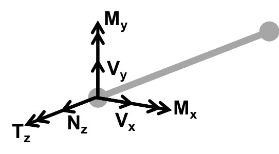
Fig. 36 Coordinate system for frame element forces.
Loads
All of the loads described above are integrated together within Frame3DD. These loads include,
Rotor-nacelle-assembly loads (thrust, moments, etc)
Mooring line force
Wind and wave loading
Gravity loads (weight distribution)
Hydrostatic pressure loads, including buoyancy
The forces, moments, and mass properties of the rotor-nacelle assembly (RNA) are inputs to FloatingSE (mass properties are assumed to be relative to the tower top position). It assumed that the RNA is a rigid body with respect to the tower modes and the mass properties, forces, and moments, are applied to the corresponding node in the model. The forces along each mooring line are applied to the connection point nodes on the structure. The wind and wave forces per unit length in Equations [eqn:drag] and [eqn:morison] are applied as trapezoidally varying loads along the column elements. Other loads applied to the structure include the gravity loads, and the buoyancy acting on the submerged elements.
Boundary Conditions
Multiple boundary conditions are applied to the structure. The mooring system stiffness matrix (linearized about the neutral position) is applied at the mooring connection nodes. However, even with the mooring stiffness, the finite element analysis would otherwise still regard the structure as unrestrained and incapable of supporting any static loads. Thus, in order to successfully compute stress and buckling limits in a well-posed problem, an additional rigid boundary condition (in all 6 DOF) is imposed at the bottom node of the main column.
Outputs
Structural analysis outputs include mass properties of the structure, member stresses, and summary forces and moments on the body. Mass properties include the total mass of the floating turbine and the mass of the substructure itself. The calculations also allow for easy computation of the center of mass of the structure (not accounting for variable ballast) and the center of buoyancy (centroid of the submerged volume). The first two natural frequencies of the structure are also computed to compare against the range of standard wave frequencies and rotor passing frequencies (1P and 3P). Next, the reaction forces and moments at the boundary node at the keel are taken as the total loading on the structure. These are used later in the static stability calculations to ensure that the mooring lines provide adequate restoring force and moment. Finally, the axial and shear forces within each frame element are extracted and converted to stresses using cross-sectional properties. These element member follow the sign convention in Fig. 36,
where \(N\) is the axial force (tension or compression), \(T\) is the torsional moment, \(V\) is the shear force, \(M\) is the bending moment, \(\sigma_z\) is the axial stress, and \(\tau_{z\theta}\) is the shear stress across axial and hoop principle directions.
Hoop stress of the tower is estimated from the dynamic pressure of the wind loads using the Eurocode method [EuropeanCfStandardisation93]. Hoop stress of the submerged columns is determined using the dynamic and static pressure heads of the water.
where \(\sigma_{\theta}\) is the hoop stress, \(q_{max}\) is the maximum dynamic pressure on a cross-section, and \(p_{hydro}\) is the hydrostatic pressure with contributions from wave motion and the static head. In the Eurocode method, \(k_w\) is the dynamic pressure factor for hoop stress calculation using cylinder dimensions and an external pressure buckling factor. Note that the argument, \((z)\), was dropped from many of the terms without losing generality.
Code Compliance as Utilizations
Once the stress components of all structural members are computed, they are compared against design code standards for compliance, and serve as design constraints when conducting optimization. Multiple code standards are used across all components. For all columns, the tower, and substructure pontoons, stress components (axial, shear, and hoop) are combined into a von Mises, equivalent, stress,
where \(\sigma_{vm}\) is the von Mises stress, \(\sigma_a\) is the axial stress, \(\tau_{a\theta}\) is the shear stress across axial and hoop principle directions. and \(\sigma_{\theta}\) is chosen as the relevant hoop stress. The von Mises stress is compared against the yield stress, \(\sigma_y\), and a safety factor as a utilization criterion.
Main column, offset column, and tower segment stresses and geometry are also evaluated against a shell buckling criterion published by [EuropeanCfStandardisation93] and a global buckling criterion published by [GermanischerLloyd05]. Note that the implementation of the Eurocode buckling is modified slightly so as to produce continuously differentiable output. See [Dam16] for a more detailed exposition.
For submerged columns, additional code standard utilization ratios are taken from the American Petroleum Institute, Bulletin 2U (specifically the procedure outlined in Appendix B) [AmericanPIAPI04]. These standards also apply shell and general buckling criterion with a margin of safety in a manner that accounts for stiffeners and the common buckling modes of submerged structures. Future efforts will also apply Bulletin 2V, the standards for plates, to the legs that support taut mooring lines.
Mooring Lines
The quasi-steady mooring system analysis is handled by the external Mooring Analysis Program (MAP++) library [MJR13], which has convenient Python bindings to access the simulation output, bundled into the WISDEM pyMAP module. MAP++ is designed to model the steady-state forces on a Multi-Segmented, Quasi-Static (MSQS) mooring line. Seabed contact, seabed friction, and multi-element mooring lines with arbitrary connection configurations can be analyzed. MAP++ inputs include sea depth, geometry descriptions of the mooring line connections, and material properties of the lines. For chain and rope-based cables, these material properties are not easily derived and would be typically provided by a manufacturer. We borrow from the approach of the popular Orcina OrcaFlex software [Orcina18] and use the following expressions,
where \(MBL\) is minimum breaking load, \(d\) is the diameter of a single half-chain link, \(A\) is the chain cross-sectional area, \(E\) is the Young’s modulus, \(EA\) is the axial stiffness. When conducting optimization, the expression for \(MBL\) is poorly posed due to its limited range of diameter applicability, so a linear fit is used instead,
Hydrostatic Stability
Neutral Buoyancy
Any floating body requires enough water displacement to create sufficient buoyancy force such that the body stays afloat in the most extreme loading and environmental conditions. This level of displacement would otherwise be overkill for more benign loading conditions. Since a floating turbine is designed for a constant hub height, variable amounts of ballast are required to maintain a neutrally buoyant system for all operating conditions. The variable ballast is simply ocean water that is pulled in or pumped out of holding areas within the substructure columns.
In FloatingSE, the variable ballast water mass is calculated as the difference between the total mass of displaced water and the total mass of the floating turbine. This mass is then divided by the water density to obtain the variable ballast volume, which is then compared to the frustum shell cross section profile above the permanent ballast to determine the height of the water ballast within the column. Once this is determined, the final center of mass of the system can be determined.
Surge/Sway Stability
Surge and sway stability is not actively tracked over the coarse of a load case. Instead the total surge force on the structure is calculated at the initial conditions and compared to the restoring force of the mooring system at the maximum allowable surge offset, which is specified by the user.
The surge direction is assumed to be aligned with the wind vector, which is aligned with the \(x\)-axis. Since the rotor yaw is assumed to be \(0^{\circ}\), the surge forces on the turbine include the rotor thrust and the wind and wave drag on the tower and substructure. The final surge force over the whole structure is taken from the \(x\)-direction reaction force of the reaction node in Frame3DD.
The restoring force is calculated as the smallest possible restoring force after a displacement in any angular direction in the mooring model. Since the alignment of the mooring lines relative to the incoming wind direction is arbitrary, a maximum offset is simulated at \(2^{\circ}\) increments around the unit circle. Also recorded in this survey is the maximum mooring line tension in any line, in any direction, for comparison against the minimum breaking load value,
where \(F_x\) is the surge force and \({\mathbb{T}}\) is the tension. If restoring force at this maximum offset is greater than the surge force applied, then the system is considered stable in surge. Since the wind and wave profiles are essentially 2-D in the \(x-z\) plane, the sway stability is given the same status as surge stability.
Pitch Stability
The approach to pitch stability determination is similar to that of surge stability. The total pitching moment on the floating turbine is calculated and compared to the restoring moment at the maximum allowable angle of heel. If the restoring moment at this max heel angle is greater than the pitching moment applied, the system is said to be statically stable in pitch.
Similar to the surge force calculation, the total pitching moment is determined from the reaction moment at the boundary condition in the Frame3DD analysis. The pitching moment has contributions from the wind and wave loads on the structure, the rotor forces and torques, the buoyancy forces on the submerged substructure, and the off-center weight of components (e.g. the RNA).
The restoring pitching moment has two primary contributions. The first is from the mooring lines. Similar to the surge force calculation, here the floating turbine is deflected in pitch by the maximum allowable heel angle and the mooring forces are recorded. The restoring moment contribution from the mooring system is computed as,
where \(r_{cm-l}\) is the vector from the center of mass to the mooring connection, and \(F_l\) is the force applied by the \(l\)-.5exmooring line. As above, \(F_l\) is taken as the minimum set over the possible orientations of the mooring lines relative to the direction.
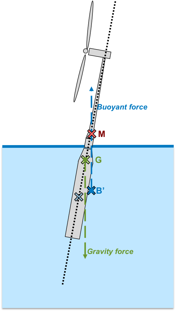
Fig. 37 Static stability of floating offshore wind turbine in neutral position.
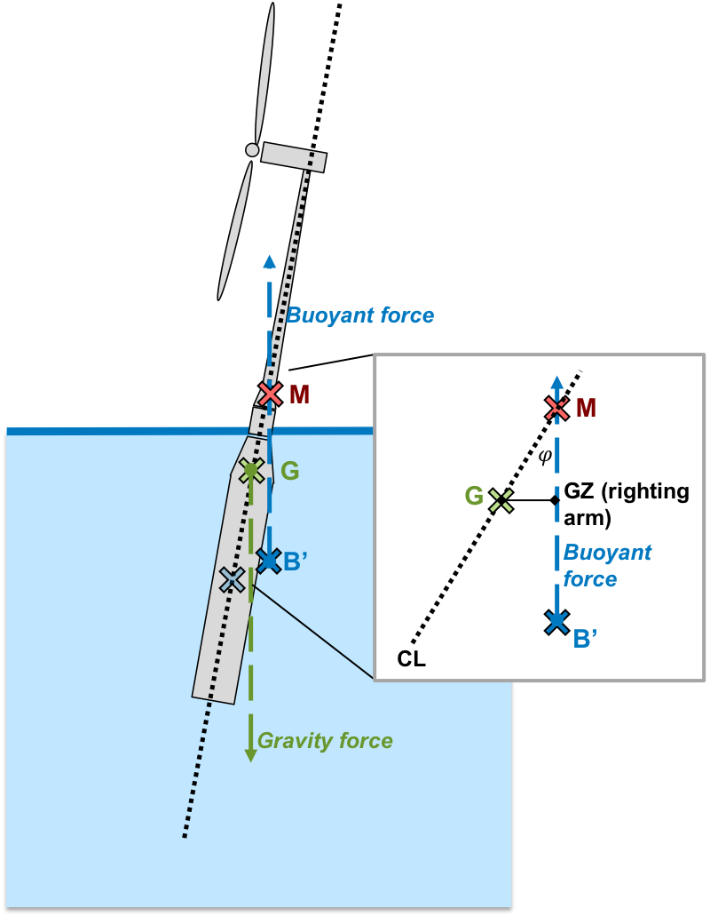
Fig. 38 Static stability of floating offshore wind turbine in pitched position.
The second contributing restoring moment comes from the motion of the center of buoyancy away from alignment with the center of mass. This is a standard calculation in naval architecture [TD14] and is diagrammed in Figure [fig:metacenter]. In this diagram, the center of mass is denoted, \(G\), the center of buoyancy is \(B\), and the metacenter is \(M\). In neutral conditions (Figure [fig:metacenter]a), all of these points are vertically aligned.
As the structure lists or heels, the center of buoyancy shifts toward the side of the structure that is more submerged (from \(B\) to \(B'\)) and the buoyancy force no longer passes through the center of mass. Instead, the buoyancy force passes through the metacenter with an effective moment arm of \(GZ\) from the center of mass (Figure [fig:metacenter]b). The metacenter is defined as the common point through which the buoyancy force acts as it pitches through small displacements, for bodies with sufficient freeboard margin.
The metacenteric height, \(GM\) is most easily calculated as an offset from the center of buoyancy (\(BM\)) by,
where \(BG\), the distance between the centers of buoyancy and gravity is easily calculated, \(I_w\) is the second moment of area of the substructure waterplane (with units of ) and \(V\) is the total volume of displacement (with units of ). Note that for semisubmersible type geometries, \(I_w\) is calculated with the parallel axis theorem for all of the columns at the waterplane,
where \(S_i\) is the waterplane cross sectional area of the \(i\)-.5excolumn and \(r_i\) is the distance from the waterplane centroid to the \(i\)-.5excolumn centroid.
The restoring moment is then the buoyancy force acting through the restoring arm, \(GZ\),
where \(\varphi\) is the angle of heel.
For this reason, the metacenter must be located above the center of mass for static stability. This condition is imposed on the design as a constraint. Note that the total volume of displacement, and the subsequent buoyancy force, is not recalculated in the perturbed configuration. It is assumed that the angles of deflection are small and that there is sufficient freeboard and design symmetry such that the total displacement is constant.
The total restoring pitching moment is then the sum of two contributions,
Hydrodynamic Stability
Floating bodies are typically modeled, for small motions and linearized behavior, as a second-order differential system with mass, damping, and spring stiffness terms,
where \({\mathbf{x}}\in{\mathbb{R}}^6\) is the six-degree of freedom vector (commonly ordered as 1-surge, 2-sway, 3-heave, 4-roll, 5-pitch, 6-yaw), \({\mathbf{M}}\) is the mass matrix, \({\mathbf{A}}\) is the added mass matrix, \({\mathbf{C}}\) is the damping matrix, and \({\mathbf{K}}\) is the stiffness matrix. The right-hand side of the equation captures the time-dependent summation of all forces.
As a low-fidelity, quasi-static sizing and cost module, FloatingSE does not attempt to capture all of the matrix entries or forcing terms of the hydrodynamics. A more sophisticated time- or frequency-domain solver, where these quantities are calculated, may be linked or included into FloatingSE in the future. Nevertheless, it does attempt to compute the diagonal entries of the mass and stiffness matrices in order to derive the rigid body natural frequencies of the system,
where \(f_i\) are the frequencies of the eigenmodes and \(\omega_i\) is the circular frequency. The mass matrix diagonal entries, \(M_{ii}\), are simply the mass and moments of inertia of the whole system,
Where the coordinate system notation is consistent with that of Figure [fig:diagram].
The added mass matrix diagonal entries are evaluated via standard strip theory for the tapered vertical columns. The added mass for the system is a summation over the columns, using the parallel axis theorem for the rotational degrees of freedom. Pontoon contributions to system added mass are currently ignored. The column quantities are calculated as,
where \(\rho\) is the water density, \(R(z)\) is the column radius along its axis, and \(V\) is the submerged volume. The extra factor of \(1/2\) in \(A_{33}\) is included to account for the fact that the top of the column extends above the waterline. Also, the integral in \(A_{55}\) is only evaluated along the submerged portion of the column.
The stiffness matrix is comprised of contributions from the mooring and hydrostatic stiffness. The mooring linearized stiffness matrix is output directly from MAP++ and needs no additional processing within FloatingSE. The hydrostatic stiffness, for a vertical column, is derived from the same principals described above regarding the metacentric height,
where \(S_{sys}\) is the waterplane area of the system.
Once the rigid body natural frequencies (eigenmodes) of the system are calculated, they are compared against the standard wave frequencies range, , and expressed as a design constraint (with a partial safety factor).
References
OrcaFlex Documentation (version 10.2b). Orcina, Durham, NC, 2018. URL: https://www.orcina.com/SoftwareProducts/OrcaFlex/Documentation.
Rick Damiani. Jacketse: an offshore wind turbine jacket sizing tool. Technical Report NREL/TP-5000-65417, National Renewable Energy Lab.(NREL), Golden, CO, February 2016. URL: https://www.nrel.gov/docs/fy16osti/65417.pdf.
Henri P. Gavin and John Pye. Frame3DD version 0.20140514+. Duke University, Durham, NC, November 2015. URL: http://frame3dd.sourceforge.net.
Marco Masciola, Jason Jonkman, and Amy Robertson. Implementation of a multisegmented, quasi-static cable model. In The Twenty-third International Offshore and Polar Engineering Conference. International Society of Offshore and Polar Engineers, 2013.
Anatol Roshko. Experiments on the flow past a circular cylinder at very high reynolds number. Journal of Fluid Mechanics, 10(3):345–356, 1961.
KP Thiagarajan and HJ Dagher. A review of floating platform concepts for offshore wind energy generation. Journal of Offshore Mechanics and Arctic Engineering, 136(2):020903, 2014.
S.P. Timoshenko and J.N. Goodier. Theory of elasticity, 3rd Edition. McGraw-Hill, 1970.
American Petroleum Institute (API). Bulletin on stability design of cylindrical shells. Technical Report API Bulletin 2U, 3rd Edition, Washington, DC, 2004.
European Committee for Standardisation. Eurocode 3: design of steel structures—part 1-6: general rules—supplementary rules for the shell structures. Technical Report EN 1993-1-6: 20xx, European Committee for Standardisation, 1993.
Germanischer Lloyd. Guideline for the certification of offshore wind turbines. Technical Report IV – Part 2, Chapter 6, Germanischer Lloyd, 2005.