4. OpenMDAO Examples
WISDEM can be run through the yaml-input files if the intention is to do a full turbine and LCOE roll-up. Sometimes though, a user might just want to evaluate or optimize a single component within WISDEM. This can also be done through the yaml-input files, and some of the examples for the tower, monopile, and drivetrain show how that is accomplished. However, for other modules it may be simpler to interface with WISDEM directly with a python script. Since WISDEM is built on top of the OpenMDAO library, this tutorial is a cursory introduction into OpenMDAO syntax and problem structure.
OpenMDAO serves to connect the various components of turbine models into a cohesive whole that can be optimized in systems engineering problems. WISDEM uses OpenMDAO to build up modular components and groups of components to represent a wind turbine. Fortunately, OpenMDAO already provides some excellent training examples on their website.
Tutorial 1: Betz Limit
This tutorial is based on the OpenMDAO example, Optimizing an Actuator Disk Model to Find Betz Limit for Wind Turbines, which we have extracted and added some additional commentary. The aim of this tutorial is to summarize the key points you’ll use to create basic WISDEM models. For those interested in WISDEM development, getting comfortable with all of the core OpenMDAO training examples is strongly encouraged.
A classic problem of wind energy engineering is the Betz limit. This is the theoretical upper limit of power that can be extracted from wind by an idealized rotor. While a full explanation is beyond the scope of this tutorial, it is explained in many places online and in textbooks. One such explanation is on Wikipedia https://en.wikipedia.org/wiki/Betz%27s_law .
Problem formulation
According to the Betz limit, the maximum power a turbine can extract from wind is:
Where \(C_p\) is the coefficient of power.
We will compute this limit using OpenMDAO by optimizing the power coefficient as a function of the induction factor (ratio of rotor plane velocity to freestream velocity) and a model of an idealized rotor using an actuator disk.
Here is our actuator disc:
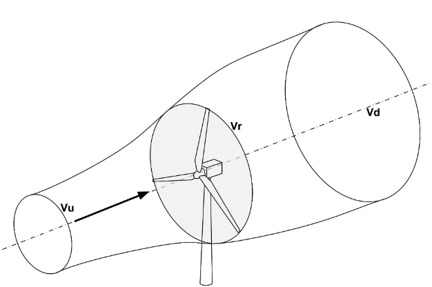
Fig. 7 Actuator disc
Where \(V_u\) freestream air velocity, upstream of rotor, \(V_r\) is air velocity at rotor exit plane and \(V_d\) is slipstream air velocity downstream of rotor, all measured in \(\frac{m}{s}\).
There are few other variables we’ll have:
\(a\): Induced Velocity Factor
Area: Rotor disc area in \(m^2\)
thrust: Thrust produced by the rotor in N
\(C_t\): Thrust coefficient
power: Power produced by rotor in W
\(\rho\): Air density in \(kg /m^3\)
Before we start in on the source code, let’s look at a few key snippets of the code
OpenMDAO implementation
First we need to import OpenMDAO
import openmdao.api as om
Now we can make an ActuatorDisc class that models the actuator disc
theory for the optimization. This is derived from an OpenMDAO class
class ActuatorDisc(om.ExplicitComponent):
    # Inputs and Outputs
    def setup(self):
        # Inputs into the the model
        self.add_input("a", 0.5, desc="Indcued velocity factor")
        self.add_input("Area", 10.0, units="m**2", desc="Rotor disc area")
        self.add_input("rho", 1.225, units="kg/m**3", desc="Air density")
        self.add_input("Vu", 10.0, units="m/s", desc="Freestream air velocity, upstream of rotor")

        # Outputs
        self.add_output("Vr", 0.0, units="m/s", desc="Air velocity at rotor exit plane")
        self.add_output("Vd", 0.0, units="m/s", desc="Slipstream air velocity, downstream of rotor")
        self.add_output("Ct", 0.0, desc="Thrust coefficient")
        self.add_output("Cp", 0.0, desc="Power coefficient")
        self.add_output("power", 0.0, units="W", desc="Power produced by the rotor")
        self.add_output("thrust", 0.0, units="m/s")

        # Declare which outputs are dependent on which inputs
        self.declare_partials("Vr", ["a", "Vu"])
        self.declare_partials("Vd", "a")
        self.declare_partials("Ct", "a")
        self.declare_partials("thrust", ["a", "Area", "rho", "Vu"])
        self.declare_partials("Cp", "a")
        self.declare_partials("power", ["a", "Area", "rho", "Vu"])
        # --------

    # Core theory
    def compute(self, inputs, outputs):
        a = inputs["a"]
        Vu = inputs["Vu"]
        rho = inputs["rho"]
        Area = inputs["Area"]
        qA = 0.5 * rho * Area * Vu**2
        outputs["Vd"] = Vd = Vu * (1 - 2 * a)
        outputs["Vr"] = 0.5 * (Vu + Vd)
        outputs["Ct"] = Ct = 4 * a * (1 - a)
        outputs["thrust"] = Ct * qA
        outputs["Cp"] = Cp = Ct * (1 - a)
        outputs["power"] = Cp * qA * Vu
        # --------

    # Derivatives of outputs wrt inputs
    def compute_partials(self, inputs, J):
        a = inputs["a"]
        Vu = inputs["Vu"]
        Area = inputs["Area"]
        rho = inputs["rho"]

        a_times_area = a * Area
        one_minus_a = 1.0 - a
        a_area_rho_vu = a_times_area * rho * Vu

        J["Vr", "a"] = -Vu
        J["Vr", "Vu"] = one_minus_a
        J["Vd", "a"] = -2.0 * Vu
        J["Ct", "a"] = 4.0 - 8.0 * a
        J["thrust", "a"] = 0.5 * rho * Vu**2 * Area * J["Ct", "a"]
        J["thrust", "Area"] = 2.0 * Vu**2 * a * rho * one_minus_a
        J["thrust", "Vu"] = 4.0 * a_area_rho_vu * one_minus_a
        J["Cp", "a"] = 4.0 * a * (2.0 * a - 2.0) + 4.0 * one_minus_a**2
        J["power", "a"] = (
            2.0 * Area * Vu**3 * a * rho * (2.0 * a - 2.0) + 2.0 * Area * Vu**3 * rho * one_minus_a**2
        )
        J["power", "Area"] = 2.0 * Vu**3 * a * rho * one_minus_a**2
        J["power", "rho"] = 2.0 * a_times_area * Vu**3 * (one_minus_a) ** 2
        J["power", "Vu"] = 6.0 * Area * Vu**2 * a * rho * one_minus_a**2
The class declaration, class ActuatorDisc(om.ExplicitComponent):
shows that our class, ActuatorDisc inherits from the
ExplicitComponent class in OpenMDAO. In WISDEM, 99% of all coded
components are of the ExplicitComponent class, so this is the most
fundamental building block to get accustomed to. Other types of
components are described in the OpenMDAO docs
here.
The ExplicitComponent class provides a template for the user to: -
Declare their input and output variables in the setup method -
Calculate the outputs from the inputs in the compute method. In an
optimization loop, this is called at every iteration. - Calculate
analytical gradients of outputs with respect to inputs in the
compute_partials method.
The variable declarations take the form of self.add_input or
self.add_output where a variable name and default/initial vaue is
assigned. The value declaration also tells the OpenMDAO internals about
the size and shape for any vector or multi-dimensional variables. Other
optional keywords that can help with code documentation and model
consistency are units= and desc=.
Working with analytical derivatives
We need to tell OpenMDAO which derivatives will need to be computed. That happens in the following lines:
        self.declare_partials("Vr", ["a", "Vu"])
        self.declare_partials("Vd", "a")
        self.declare_partials("Ct", "a")
        self.declare_partials("thrust", ["a", "Area", "rho", "Vu"])
        self.declare_partials("Cp", "a")
        self.declare_partials("power", ["a", "Area", "rho", "Vu"])
Note that lines like self.declare_partials('Vr', ['a', 'Vu'])
references both the derivatives \(\partial `V_r /
:math:\)partial a and \(\partial `V_r /
:math:\)partial V_u.
The Jacobian in which we provide solutions to the derivatives is
    def compute_partials(self, inputs, J):
        a = inputs["a"]
        Vu = inputs["Vu"]
        Area = inputs["Area"]
        rho = inputs["rho"]

        a_times_area = a * Area
        one_minus_a = 1.0 - a
        a_area_rho_vu = a_times_area * rho * Vu

        J["Vr", "a"] = -Vu
        J["Vr", "Vu"] = one_minus_a
        J["Vd", "a"] = -2.0 * Vu
        J["Ct", "a"] = 4.0 - 8.0 * a
        J["thrust", "a"] = 0.5 * rho * Vu**2 * Area * J["Ct", "a"]
        J["thrust", "Area"] = 2.0 * Vu**2 * a * rho * one_minus_a
        J["thrust", "Vu"] = 4.0 * a_area_rho_vu * one_minus_a
        J["Cp", "a"] = 4.0 * a * (2.0 * a - 2.0) + 4.0 * one_minus_a**2
        J["power", "a"] = (
            2.0 * Area * Vu**3 * a * rho * (2.0 * a - 2.0) + 2.0 * Area * Vu**3 * rho * one_minus_a**2
        )
        J["power", "Area"] = 2.0 * Vu**3 * a * rho * one_minus_a**2
        J["power", "rho"] = 2.0 * a_times_area * Vu**3 * (one_minus_a) ** 2
        J["power", "Vu"] = 6.0 * Area * Vu**2 * a * rho * one_minus_a**2
In OpenMDAO, multiple components can be connected together inside of a Group. There will be some other new elements to review, so let’s take a look:
Betz Group:
class Betz(om.Group):
    """
    Group containing the actuator disc equations for deriving the Betz limit.
    """

    def setup(self):
        indeps = self.add_subsystem("indeps", om.IndepVarComp(), promotes=["*"])
        indeps.add_output("a", 0.5)
        indeps.add_output("Area", 10.0, units="m**2")
        indeps.add_output("rho", 1.225, units="kg/m**3")
        indeps.add_output("Vu", 10.0, units="m/s")

        self.add_subsystem("a_disk", ActuatorDisc(), promotes=["a", "Area", "rho", "Vu"])
The Betz class derives from the OpenMDAO Group class, which is
typically the top-level class that is used in an analysis. The OpenMDAO
Group class allows you to cluster models in hierarchies. We can put
multiple components in groups. We can also put other groups in groups.
Components are added to groups with the self.add_subsystem command,
which has two primary arguments. The first is the string name to call
the subsystem that is added and the second is the component or sub-group
class instance. A common optional argument is promotes=, which
elevates the input/output variable string names to the top-level
namespace. The Betz group shows examples where the promotes= can
be passed a list of variable string names or the '*' wildcard to
mean all input/output variables.
The first subsystem that is added is an IndepVarComp, which are the
independent variables of the problem. Subsystem inputs that are not tied
to other subsystem outputs should be connected to an independent
variables. For optimization problems, design variables must be part of
an IndepVarComp. In the Betz problem, we have a, Area,
rho, and Vu. Note that they are promoted to the top level
namespace, otherwise we would have to access them by 'indeps.x' and
'indeps.z'.
The next subsystem that is added is an instance of the component we created above:
self.add_subsystem('a_disk', ActuatorDisc(), promotes=['a', 'Area', 'rho', 'Vu'])
The promotes= can also serve to connect variables. In OpenMDAO, two
variables with the same string name in the same namespace are
automatically connected. By promoting the same variable string names as
in the IndepCarComp, they are automatically connected. For variables
that are not connected in this way, explicit connect statements are
required, which is demonstrated in the next tutorial. ## Let’s optimize
our system!
Even though we have all the pieces in a Group, we still need to put
them into a Problem to be executed. The Problem instance is
where we can assign design variables, objective functions, and
constraints. It is also how the user interacts with the Group to set
initial conditions and interrogate output values.
First, we instantiate the Problem and assign an instance of Betz
to be the root model:
prob = om.Problem()
prob.model = Betz()
Next we assign an optimization driver to the problem instance. If we only wanted to evaluate the model once and not optimize, then a driver is not needed:
prob.driver = om.ScipyOptimizeDriver()
prob.driver.options["optimizer"] = "SLSQP"
With the optimization driver in place, we can assign design variables, objective(s), and constraints. Any IndepVarComp can be a design variable and any model output can be an objective or constraint.
We want to maximize the objective, but OpenMDAO will want to minimize it
as it is consistent with the standard optimization problem statement. So
we minimize the negative to find the maximum. Note that Cp is not
promoted from a_disk. Therefore we must reference it with
a_disk.Cp
prob.model.add_design_var("a", lower=0.0, upper=1.0)
prob.model.add_design_var("Area", lower=0.0, upper=1.0)
prob.model.add_objective("a_disk.Cp", scaler=-1.0)
Now we can run the optimization:
prob.setup()
prob.run_driver()
Optimization terminated successfully.    (Exit mode 0)
            Current function value: -0.5925925906659251
            Iterations: 5
            Function evaluations: 6
            Gradient evaluations: 5
Optimization Complete
-----------------------------------
Finally, the result:
Above, we see a summary of the steps in our optimization. Next, we print out the values we care about and list all of the inputs and outputs that are problem used.
print("Coefficient of power Cp = ", prob["a_disk.Cp"])
print("Induction factor a =", prob["a"])
print("Rotor disc Area =", prob["Area"], "m^2")
prob.model.list_inputs(units=True)
prob.model.list_outputs(units=True)
Coefficient of power Cp =  [0.59259259]
Induction factor a = [0.33335528]
Rotor disc Area = [1.] m^2
4 Input(s) in 'model'
---------------------

varname   value
--------  ------------
top
  a_disk
    a     [0.33335528]
    Area  [1.]
    rho   [1.225]
    Vu    [10.]


10 Explicit Output(s) in 'model'
--------------------------------

varname     value
----------  --------------
top
  indeps
    a       [0.33335528]
    Area    [1.]
    rho     [1.225]
    Vu      [10.]
  a_disk
    Vr      [6.6664472]
    Vd      [3.33289439]
    Ct      [0.88891815]
    Cp      [0.59259259]
    power   [362.96296178]
    thrust  [54.44623668]


0 Implicit Output(s) in 'model'
-------------------------------
And there we have it. This matched the Betz limit of:
Tutorial 2. The Sellar Problem
This tutorial is based on the OpenMDAO example, Sellar - A Two-Discipline Problem with a Nonlinear Solver, which we have extracted and added some additional commentary. The aim of this tutorial is to summarize the key points needed to create or understand basic WISDEM models. For those interested in WISDEM development, getting comfortable with all of the core OpenMDAO training examples is strongly encouraged.
Problem formulation
The Sellar problem are a couple of components (what Wikipedia calls models) that are simple equations. There is an objective to optimize and a couple of constraints to follow.
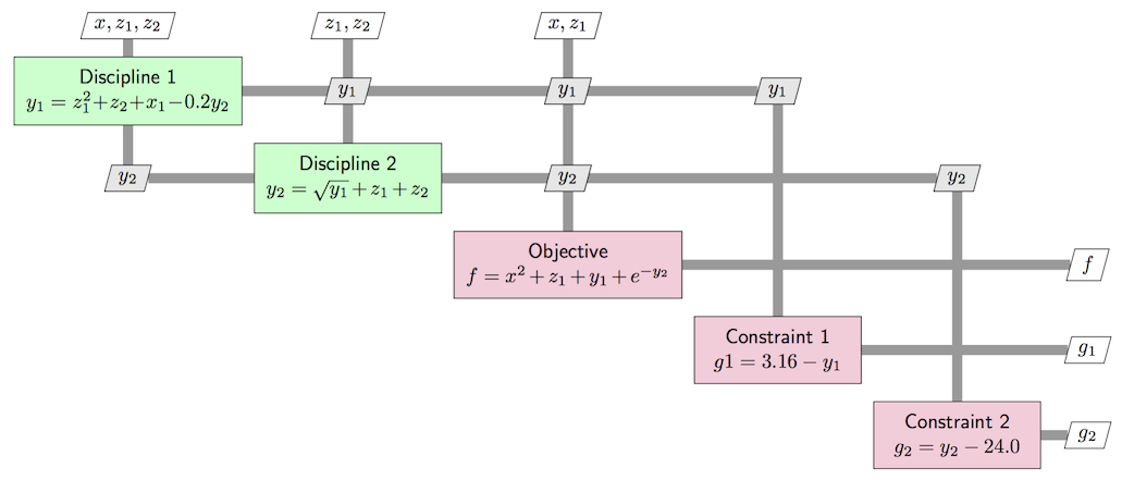
Fig. 8 Sellar XDSM
This is an XDSM diagram that is used to describe the problem and optimization setups. For more reference on this notation and general reference for multidisciplinary design analysis and optimization (MDAO), see:
Problem formulation section of multidisciplinary design optimization on Wikipedia: Read the definitions for design variables, constraints, objectives and models.
Lambe and Martins: Extensions to the Design Structure Matrix for the Description of Multidisciplinary Design, Analysis, and Optimization Processes: Read section 2 “Terminology and Notation” for further explanation of design variables, discipline analysis, response variables, target variables and coupling variables. Read section 4 about XDSM diagrams that describe MDO processes.
OpenMDAO implementation
First we need to import OpenMDAO
import numpy as np
import openmdao.api as om
Let’s build Discipline 1 first. On the XDSM diagram, notice the parallelograms connected to Discipline 1 by thick grey lines. These are variables pertaining to the Discipline 1 component.
\(\mathbf{z}\): An input. Since the components \(z_1, z_2\) can form a vector, we call the variable
zin the code and initialize it to \((0, 0)\) withnp.zeros(2). Note that components of \(\mathbf{z}\) are found in 3 of the white \(\mathbf{z}\) parallelograms connected to multiple components and the objective, so this is a global design variable.\(x\): An input. A local design variable for Discipline 1. Since it isn’t a vector, we just initialize it as a float.
\(y_2\): An input. This is a coupling variable coming from an output on Discipline 2
\(y_1\): An output. This is a coupling variable going to an input on Discipline 2
Let’s take a look at the Discipline 1 component and break it down piece by piece. ### Discipline 1
class SellarDis1(om.ExplicitComponent):
    """
    Component containing Discipline 1 -- no derivatives version.
    """

    def setup(self):
        # Global Design Variable
        self.add_input("z", val=np.zeros(2))

        # Local Design Variable
        self.add_input("x", val=0.0)

        # Coupling parameter
        self.add_input("y2", val=1.0)

        # Coupling output
        self.add_output("y1", val=1.0)

        # Finite difference all partials.
        self.declare_partials("*", "*", method="fd")

    def compute(self, inputs, outputs):
        """
        Evaluates the equation
        y1 = z1**2 + z2 + x1 - 0.2*y2
        """
        z1 = inputs["z"][0]
        z2 = inputs["z"][1]
        x1 = inputs["x"]
        y2 = inputs["y2"]

        outputs["y1"] = z1**2 + z2 + x1 - 0.2 * y2
The class declaration, class SellarDis1(om.ExplicitComponent): shows
that our class, SellarDis1 inherits from the ExplicitComponent
class in OpenMDAO. In WISDEM, 99% of all coded components are of the
ExplicitComponent class, so this is the most fundamental building
block to get accustomed to. Keen observers will notice that the Sellar
Problem has implicitly defined variables that will need to be
addressed, but that is addressed below. Other types of components are
described in the OpenMDAO docs
here.
The ExplicitComponent class provides a template for the user to: -
Declare their input and output variables in the setup method -
Calculate the outputs from the inputs in the compute method. In an
optimization loop, this is called at every iteration. - Calculate
analytical gradients of outputs with respect to inputs in the
compute_partials method. This is absent from the Sellar Problem.
The variable declarations take the form of self.add_input or
self.add_output where a variable name and default/initial vaue is
assigned. The value declaration also tells the OpenMDAO internals about
the size and shape for any vector or multi-dimensional variables. Other
optional keywords that can help with code documentation and model
consistency are units= and desc=.
Finally self.declare_partials('*', '*', method='fd') tell OpenMDAO
to use finite difference to compute the partial derivative of the
outputs with respect to the inputs. OpenMDAO provides many finite
difference capabilities including: - Forward and backward differencing -
Central differencing for second-order accurate derivatives -
Differencing in the complex domain which can offer improved accuracy for
the models that support it
Now lets take a look at Discipline 2.
\(\mathbf{z}\): An input comprised of \(z_1, z_2\).
\(y_2\): An output. This is a coupling variable going to an input on Discipline 1
\(y_1\): An input. This is a coupling variable coming from an output on Discipline 1
Discipline 2
class SellarDis2(om.ExplicitComponent):
    """
    Component containing Discipline 2 -- no derivatives version.
    """

    def setup(self):
        # Global Design Variable
        self.add_input("z", val=np.zeros(2))

        # Coupling parameter
        self.add_input("y1", val=1.0)

        # Coupling output
        self.add_output("y2", val=1.0)

        # Finite difference all partials.
        self.declare_partials("*", "*", method="fd")

    def compute(self, inputs, outputs):
        """
        Evaluates the equation
        y2 = y1**(.5) + z1 + z2
        """

        z1 = inputs["z"][0]
        z2 = inputs["z"][1]
        y1 = inputs["y1"]

        outputs["y2"] = y1**0.5 + z1 + z2
In OpenMDAO, multiple components can be connected together inside of a Group. There will be some other new elements to review, so let’s take a look:
Sellar Group:
class SellarMDA(om.Group):
    """
    Group containing the Sellar MDA.
    """

    def setup(self):
        indeps = self.add_subsystem("indeps", om.IndepVarComp(), promotes=["*"])
        indeps.add_output("x", 1.0)
        indeps.add_output("z", np.array([5.0, 2.0]))

        self.add_subsystem("d1", SellarDis1(), promotes=["y1", "y2"])
        self.add_subsystem("d2", SellarDis2(), promotes=["y1", "y2"])
        self.connect("x", "d1.x")
        self.connect("z", ["d1.z", "d2.z"])

        # Nonlinear Block Gauss Seidel is a gradient free solver to handle implicit loops
        self.nonlinear_solver = om.NonlinearBlockGS()

        self.add_subsystem(
            "obj_cmp",
            om.ExecComp("obj = x**2 + z[1] + y1 + exp(-y2)", z=np.array([0.0, 0.0]), x=0.0),
            promotes=["x", "z", "y1", "y2", "obj"],
        )

        self.add_subsystem("con_cmp1", om.ExecComp("con1 = 3.16 - y1"), promotes=["con1", "y1"])
        self.add_subsystem("con_cmp2", om.ExecComp("con2 = y2 - 24.0"), promotes=["con2", "y2"])
The SellarMDA class derives from the OpenMDAO Group class,
which is typically the top-level class that is used in an analysis. The
OpenMDAO Group class allows you to cluster models in hierarchies. We
can put multiple components in groups. We can also put other groups in
groups.
Components are added to groups with the self.add_subsystem command,
which has two primary arguments. The first is the string name to call
the subsystem that is added and the second is the component or sub-group
class instance. A common optional argument is promotes=, which
elevates the input/output variable string names to the top-level
namespace. The SellarMDA group shows examples where the
promotes= can be passed a list of variable string names or the
'*' wildcard to mean all input/output variables.
The first subsystem that is added is an IndepVarComp, which are the
independent variables of the problem. Subsystem inputs that are not tied
to other subsystem outputs should be connected to an independent
variables. For optimization problems, design variables must be part of
an IndepVarComp. In the Sellar problem, we have x and z.
Note that they are promoted to the top level namespace, otherwise we
would have to access them by 'indeps.x' and 'indeps.z'.
The next subsystems that are added are instances of the components we created above:
self.add_subsystem('d1', SellarDis1(), promotes=['y1', 'y2'])
self.add_subsystem('d2', SellarDis2(), promotes=['y1', 'y2'])
The promotes= can also serve to connect variables. In OpenMDAO, two
variables with the same string name in the same namespace are
automatically connected. By promoting y1 and y2 in both d1
and d2, they are automatically connected. For variables that are not
connected in this way, explicit connect statements are required such as:
self.connect('x', ['d1.x','d2.x'])
self.connect('z', ['d1.z','d2.z'])
These statements connect the IndepVarComp versions of x and
z to the d1 and d2 versions. Note that if x and z
could easily have been promoted in d1 and d2 too, which would
have made these connect statements unnecessary, but including them is
instructive.
The next statement, self.nonlinear_solver = om.NonlinearBlockGS(),
handles the required internal iteration between y1 and y2 is our
two components. OpenMDAO is able to identify a cycle between
input/output variables and requires the user to specify a solver to
handle the nested iteration loop. WISDEM does its best to avoid cycles.
Finally, we have a series of three subsystems that use instances of the
OpenMDAO ExecComp component. This is a useful way to defining an
ExplicitComponent inline, without having to create a whole new
class. OpenMDAO is able to parse the string expression and populate the
setup and compute methods automatically. This technique is used
to create our objective function and two constraint functions directly:
self.add_subsystem('obj_cmp', om.ExecComp('obj = x**2 + z[1] + y1 + exp(-y2)',
                                          z=np.array([0.0, 0.0]), x=0.0),
                   promotes=['x', 'z', 'y1', 'y2', 'obj'])
self.add_subsystem('con_cmp1', om.ExecComp('con1 = 3.16 - y1'), promotes=['con1', 'y1'])
self.add_subsystem('con_cmp2', om.ExecComp('con2 = y2 - 24.0'), promotes=['con2', 'y2'])
Let’s optimize our system!
Even though we have all the pieces in a Group, we still need to put
them into a Problem to be executed. The Problem instance is
where we can assign design variables, objective functions, and
constraints. It is also how the user interacts with the Group to set
initial conditions and interrogate output values.
First, we instantiate the Problem and assign an instance of
SellarMDA to be the root model:
prob = om.Problem()
prob.model = SellarMDA()
Next we assign an optimization driver to the problem instance. If we
only wanted to evaluate the model once and not optimize, then a
driver is not needed:
prob.driver = om.ScipyOptimizeDriver()
prob.driver.options["optimizer"] = "SLSQP"
prob.driver.options["tol"] = 1e-8
With the optimization driver in place, we can assign design variables,
objective(s), and constraints. Any IndepVarComp can be a design
variable and any model output can be an objective or constraint.
prob.model.add_design_var("x", lower=0, upper=10)
prob.model.add_design_var("z", lower=0, upper=10)
prob.model.add_objective("obj")
prob.model.add_constraint("con1", upper=0)
prob.model.add_constraint("con2", upper=0)

# Ask OpenMDAO to finite-difference across the whole model to compute the total gradients for the optimizer
# The other approach would be to finite-difference for the partials and build up the total derivative
prob.model.approx_totals()
Now we are ready for to ask OpenMDAO to setup the model, to use finite differences for gradient approximations, and to run the driver:
prob.setup()
prob.run_driver()

print("minimum found at")
print(float(prob["x"]))
print(prob["z"])
print("minimum objective")
print(float(prob["obj"]))
NL: NLBGS Converged in 7 iterations
NL: NLBGS Converged in 0 iterations
NL: NLBGS Converged in 3 iterations
NL: NLBGS Converged in 4 iterations
NL: NLBGS Converged in 4 iterations
NL: NLBGS Converged in 8 iterations
NL: NLBGS Converged in 3 iterations
NL: NLBGS Converged in 4 iterations
NL: NLBGS Converged in 4 iterations
NL: NLBGS Converged in 9 iterations
NL: NLBGS Converged in 4 iterations
NL: NLBGS Converged in 5 iterations
NL: NLBGS Converged in 4 iterations
NL: NLBGS Converged in 9 iterations
NL: NLBGS Converged in 4 iterations
NL: NLBGS Converged in 5 iterations
NL: NLBGS Converged in 4 iterations
NL: NLBGS Converged in 8 iterations
NL: NLBGS Converged in 4 iterations
NL: NLBGS Converged in 5 iterations
NL: NLBGS Converged in 4 iterations
NL: NLBGS Converged in 5 iterations
NL: NLBGS Converged in 4 iterations
NL: NLBGS Converged in 5 iterations
NL: NLBGS Converged in 4 iterations
Optimization terminated successfully.    (Exit mode 0)
            Current function value: 3.183393951735934
            Iterations: 6
            Function evaluations: 6
            Gradient evaluations: 6
Optimization Complete
-----------------------------------
minimum found at
0.0
[1.97763888e+00 2.83540724e-15]
minimum objective
3.183393951735934