5. Tower and Monopile Example
In this example we show how to perform simulation and optimization of a land-based tower and an offshore tower-monopile combination. Both examples can be executed either by limiting the input yaml to only the necessary components or by using a python script that calls WISDEM directly.
Land-based Tower Design
The following example, demonstrates how to set up and run analysis or optimization for a land-based tower. Some of the geometric parameters are seen in Figure 9. The tower is not restricted to 3 sections, any number of sections can be defined.
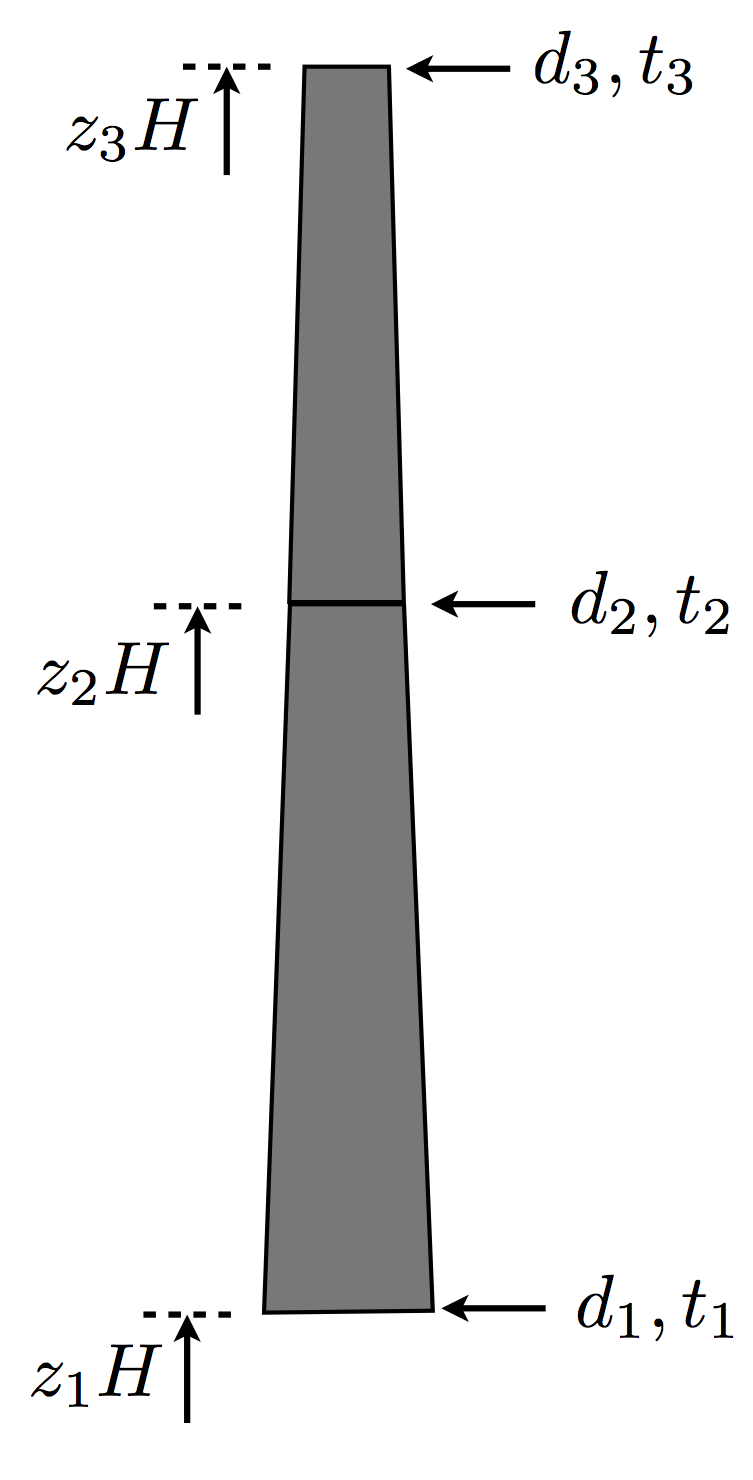
Fig. 9 Example of tower geometric parameterization.
Invoking with YAML files
To run just the tower analysis from the YAML input files, we just need to include the necessary elements. First dealing with the geometry_option.yaml file, this always includes the assembly section. Of the components, this means just the tower section. Also, the materials, environment, and costs section,
name: 5MW Tower only

assembly:
    turbine_class: I
    turbulence_class: B
    drivetrain: Geared
    rotor_orientation: Upwind
    number_of_blades: 3
    hub_height: 90.
    rotor_diameter: 126.
    rated_power: 5.e+6

components:
    tower:
        outer_shape_bem:
            reference_axis: &ref_axis_tower
                x:
                    grid: [0.0, 1.0]
                    values: [0.0, 0.0]
                y:
                    grid: [0.0, 1.0]
                    values: [0.0, 0.0]
                z:
                    grid: &grid_tower [0., 0.5, 1.]
                    values: [0., 43.8, 87.6]
            outer_diameter:
                grid: *grid_tower
                values: [6., 4.935, 3.87]
            drag_coefficient:
                grid: [0.0, 1.0]
                values: [1.0, 1.0]
        internal_structure_2d_fem:
            outfitting_factor: 1.07
            reference_axis: *ref_axis_tower
            layers:
                - name: tower_wall
                  material: steel
                  thickness:
                    grid: *grid_tower
                    values: [0.027, 0.0222, 0.019]

materials:
   -  name: steel
      description: Steel of the tower and monopile, ASTM A572 Grade 50
      source: http://www.matweb.com/search/DataSheet.aspx?MatGUID=9ced5dc901c54bd1aef19403d0385d7f
      orth: 0
      rho: 7800
      alpha: 0.0
      E: 200.e+009
      nu: 0.265
      G: 79.3e+009
      GIc: 0  #Place holder, currently not used
      GIIc: 0  #Place holder, currently not used
      alp0: 0  #Place holder, currently not used
      Xt: 1.12e+9
      Xc: 2.16e+9
      S: 0
      Xy: 345.e+6
      m: 3
      A: 3.5534648443719767e10
      unit_cost: 0.7

environment:
    air_density: 1.225
    air_dyn_viscosity: 1.81e-5
    weib_shape_parameter: 2.
    air_speed_sound: 340.
    shear_exp: 0.2
    water_density: 1025.0
    water_dyn_viscosity: 1.3351e-3
    #water_depth: 0.0
    significant_wave_height: 0.0
    significant_wave_period: 0.0
    soil_shear_modulus: 140.e+6
    soil_poisson: 0.4
costs:
    labor_rate: 58.8
    painting_rate: 30.0
The modeling_options.yaml file is also limited to just the sections we need. Note that even though the monopile options are included here, since there was no specification of a monopile in the geometry inputs, this will be ignored. One new section is added here, a loading section that specifies the load scenarios that are applied to the tower. Since there is no rotor simulation to generate the loads, they must be specified by the user directly. Note that two load cases are specified. This creates a set of constraints for both of them.
# Generic modeling options file to run standard WISDEM case
General:
    verbosity: False  # When set to True, the code prints to screen many infos
WISDEM:
    n_dlc: 2           # Number of design load cases
    RotorSE:
        flag: False
    DriveSE:
        flag: False
    TowerSE:             # Options of TowerSE module
        flag: True
        wind: PowerWind  # Wind used
        gamma_f: 1.35    # Safety factor for fatigue loads
        gamma_m: 1.3     # Safety factor for material properties
        gamma_n: 1.0     # Safety factor for ...
        gamma_b: 1.1     # Safety factor for ...
        gamma_fatigue: 1.755  # Safety factor for fatigue loads
        buckling_method: eurocode # Buckling code type [eurocode or dnvgl]
        buckling_length: 15    # Buckling parameter
        frame3dd:
            shear: True
            geom: True
            tol: 1e-9
    FixedBottomSE:
        flag: False
    BOS:
        flag: False

    Loading:
        mass: 285598.8
        center_of_mass: [-1.13197635, 0.0, 0.50875268]
        moment_of_inertia: [1.14930678e08, 2.20354030e07, 1.87597425e07, 0.0, 5.03710467e05, 0.0]
        loads:
            - force: [1284744.19620519, 0.0, -2914124.84400512]
              moment: [3963732.76208099, -2275104.79420872, -346781.68192839]
              velocity: 11.73732
            - force: [930198.60063279, 0.0, -2883106.12368949]
              moment: [-1683669.22411597, -2522475.34625363, 147301.97023764]
              velocity: 70.0
The analysis_options.yaml poses the optimization problem,
general:
    folder_output: outputs
    fname_output: tower_output
design_variables:

  tower:
    outer_diameter:
      flag: True
      lower_bound: 3.87
      upper_bound: 9.0
    layer_thickness:
      flag: True
      lower_bound: 4e-3
      upper_bound: 2e-1

merit_figure: tower_mass

constraints:
  tower:
    height_constraint:
      flag: False
      lower_bound: 1.e-2
      upper_bound: 1.e-2
    stress:
      flag: True
    global_buckling:
      flag: True
    shell_buckling:
      flag: True
    d_to_t:
      flag: True
      lower_bound: 80.0
      upper_bound: 500.0
    taper:
      flag: True
      lower_bound: 0.2
    slope:
      flag: True
    frequency_1:
      flag: True
      lower_bound: 0.13
      upper_bound: 0.40

driver:
    optimization:
        flag: True         # Flag to enable optimization
        tol: 1.e-6          # Optimality tolerance
        # max_major_iter: 10  # Maximum number of major design iterations (SNOPT)
        # max_minor_iter: 100 # Maximum number of minor design iterations (SNOPT)
        max_iter: 1         # Maximum number of iterations (SLSQP)
        solver: SLSQP       # Optimization solver. Other options are 'SLSQP' - 'CONMIN'
        step_size: 1.e-6    # Step size for finite differencing
        form: forward       # Finite differencing mode, either forward or central
    design_of_experiments:
        flag: False           # Flag to enable design of experiments
        run_parallel: True    # Flag to run using parallel processing
        generator: Uniform    # Type of input generator. (Uniform)
        num_samples: 5        # number of samples for (Uniform only)

recorder:
    flag: True              # Flag to activate OpenMDAO recorder
    file_name: log_opt.sql  # Name of OpenMDAO recorder
The yaml files can be called directly from the command line, or via a python script that passes them to the top-level WISDEM function,
$ wisdem nrel5mw_tower.yaml modeling_options.yaml analysis_options.yaml
or
$ python tower_driver.py
Where the contents of tower_driver.py are,
import os

from wisdem import run_wisdem

mydir = os.path.dirname(os.path.realpath(__file__))  # get path to this file
fname_wt_input = mydir + os.sep + "nrel5mw_tower.yaml"
fname_modeling_options = mydir + os.sep + "modeling_options.yaml"
fname_analysis_options = mydir + os.sep + "analysis_options.yaml"

wt_opt, analysis_options, opt_options = run_wisdem(fname_wt_input, fname_modeling_options, fname_analysis_options)
Calling Python Directly
The tower optimization can also be written using direct calls to WISDEM’s TowerSE module. First, we import the modules we want to use and setup the tower configuration. We set flags for if we want to perform analysis or optimization, as well as if we want plots to be shown at the end. Next, we set the tower height, diameter, and wall thickness.
# Optimization by flag
# Two load cases
import os

import numpy as np
import openmdao.api as om

from wisdem.towerse.tower import TowerSE
from wisdem.commonse.fileIO import save_data

# Set analysis and optimization options and define geometry
plot_flag = False
opt_flag = True

n_control_points = 3
n_materials = 1
n_load_cases = 2

h_param = np.diff(np.linspace(0.0, 87.6, n_control_points))
d_param = np.linspace(8.0, 3.87, n_control_points)
t_param = np.linspace(0.08, 0.02, n_control_points)
max_diam = 9.0
We then set many analysis options for the tower, including materials, safety factors, and FEM settings. The module uses the frame finite element code Frame3DD to perform the FEM analysis.
modeling_options = {}
modeling_options["flags"] = {}
modeling_options["materials"] = {}
modeling_options["materials"]["n_mat"] = n_materials
modeling_options["General"] = {}
modeling_options["WISDEM"] = {}
modeling_options["WISDEM"]["n_dlc"] = n_load_cases
modeling_options["WISDEM"]["TowerSE"] = {}
modeling_options["WISDEM"]["TowerSE"]["buckling_method"] = "eurocode"
modeling_options["WISDEM"]["TowerSE"]["buckling_length"] = 15.0
modeling_options["WISDEM"]["TowerSE"]["n_refine"] = 3

# safety factors
modeling_options["WISDEM"]["TowerSE"]["gamma_f"] = 1.35
modeling_options["WISDEM"]["TowerSE"]["gamma_m"] = 1.3
modeling_options["WISDEM"]["TowerSE"]["gamma_n"] = 1.0
modeling_options["WISDEM"]["TowerSE"]["gamma_b"] = 1.1
modeling_options["WISDEM"]["TowerSE"]["gamma_fatigue"] = 1.35 * 1.3 * 1.0

# Frame3DD options
modeling_options["WISDEM"]["TowerSE"]["frame3dd"] = {}
modeling_options["WISDEM"]["TowerSE"]["frame3dd"]["shear"] = True
modeling_options["WISDEM"]["TowerSE"]["frame3dd"]["geom"] = True
modeling_options["WISDEM"]["TowerSE"]["frame3dd"]["tol"] = 1e-9
modeling_options["WISDEM"]["TowerSE"]["frame3dd"]["modal_method"] = 1

modeling_options["WISDEM"]["TowerSE"]["n_height"] = n_control_points
modeling_options["WISDEM"]["TowerSE"]["n_layers"] = 1
modeling_options["WISDEM"]["TowerSE"]["wind"] = "PowerWind"
Next, we instantiate the OpenMDAO problem and add a tower model to this problem.
prob = om.Problem(reports=False)
prob.model = TowerSE(modeling_options=modeling_options)
Next, the script proceeds to set-up the design optimization problem if opt_flag is set to True.
In this case, the optimization driver is first be selected and configured.
We then set the objective, in this case tower mass, and scale it so it is of order 1 for better convergence behavior.
The tower diameters and thicknesses are added as design variables.
Finally, constraints are added.
Some constraints are based on the tower geometry and others are based on the stress and buckling loads experienced in the loading cases.
if opt_flag:
    # Choose the optimizer to use
    prob.driver = om.ScipyOptimizeDriver()
    prob.driver.options["optimizer"] = "SLSQP"

    # Add objective
    prob.model.add_objective("tower_mass", scaler=1e-6)

    # Add design variables, in this case the tower diameter and wall thicknesses
    prob.model.add_design_var("tower_outer_diameter_in", lower=3.87, upper=max_diam)
    prob.model.add_design_var("tower_layer_thickness", lower=4e-3, upper=2e-1)

    # Add constraints on the tower design
    prob.model.add_constraint("post.constr_stress", upper=1.0)
    prob.model.add_constraint("post.constr_global_buckling", upper=1.0)
    prob.model.add_constraint("post.constr_shell_buckling", upper=1.0)
    prob.model.add_constraint("constr_d_to_t", lower=80.0, upper=500.0)
    prob.model.add_constraint("constr_taper", lower=0.2)
    prob.model.add_constraint("slope", upper=1.0)
    prob.model.add_constraint("tower.f1", lower=0.13, upper=0.40)
We then call setup() on the OpenMDAO problem, which finalizes the components and groups for the tower analysis or optimization.
Once setup() has been called, we can access the problem values or modify them for a given analysis.
prob.setup()
Now that we’ve set up the tower problem, we set values for tower, soil, and RNA assembly properties. For the soil, shear and modulus properties for the soil can be defined, but in this example we assume that all directions are rigid (3 translation and 3 rotation). The center of mass locations are defined relative to the tower top in the yaw-aligned coordinate system. Blade and hub moments of inertia should be defined about the hub center, nacelle moments of inertia are defined about the center of mass of the nacelle.
prob["hub_height"] = prob["tower_height"] = h_param.sum()
prob["foundation_height"] = 0.0
prob["tower_s"] = np.cumsum(np.r_[0.0, h_param]) / h_param.sum()
prob["tower_outer_diameter_in"] = d_param
prob["tower_layer_thickness"] = t_param.reshape((1, -1))
prob["outfitting_factor_in"] = 1.07
prob["yaw"] = 0.0

# material properties
prob["E_mat"] = 210e9 * np.ones((n_materials, 3))
prob["G_mat"] = 80.8e9 * np.ones((n_materials, 3))
prob["rho_mat"] = [8500.0]
prob["sigma_y_mat"] = [450e6]
prob["sigma_ult_mat"] = 600e6 * np.ones((n_materials, 3))
prob["wohler_exp_mat"] = [10.0]
prob["wohler_A_mat"] = [10.0]

# extra mass from RNA
prob["rna_mass"] = np.array([285598.8])
mIxx = 1.14930678e08
mIyy = 2.20354030e07
mIzz = 1.87597425e07
mIxy = 0.0
mIxz = 5.03710467e05
mIyz = 0.0
prob["rna_I"] = np.array([mIxx, mIyy, mIzz, mIxy, mIxz, mIyz])
prob["rna_cg"] = np.array([-1.13197635, 0.0, 0.50875268])
For the power-law wind profile, the only parameter needed is the shear exponent. In addition, some geometric parameters for the wind profile’s extend must be defined, the base (or no-slip location) at z0, and the height at which a reference velocity will be defined.
prob["unit_cost_mat"] = [2.0]  # USD/kg
prob["labor_cost_rate"] = 100.0 / 60.0  # USD/min
prob["painting_cost_rate"] = 30.0  # USD/m^2

# wind & wave values
prob["wind_reference_height"] = 90.0
prob["z0"] = 0.0
prob["cd_usr"] = -1.0
prob["rho_air"] = 1.225
prob["mu_air"] = 1.7934e-5
prob["beta_wind"] = 0.0
if modeling_options["WISDEM"]["TowerSE"]["wind"] == "PowerWind":
    prob["shearExp"] = 0.2
As mentioned earlier, we are allowing for two separate loading cases. The wind speed, and rotor force/moments for those two cases are now defined. The wind speed location corresponds to the reference height defined previously as wind_zref. In this simple case, we include only thrust and torque, but in general all 3 components of force and moments can be defined in the hub-aligned coordinate system. The assembly automatically handles translating the forces and moments defined at the rotor to the tower top.
prob["env1.Uref"] = 11.73732
Fx1 = 1284744.19620519
Fy1 = 0.0
Fz1 = -2914124.84400512
Mxx1 = 3963732.76208099
Myy1 = -2275104.79420872
Mzz1 = -346781.68192839
prob["env2.Uref"] = 70.0
Fx2 = 930198.60063279
Fy2 = 0.0
Fz2 = -2883106.12368949
Mxx2 = -1683669.22411597
Myy2 = -2522475.34625363
Mzz2 = 147301.97023764
We can now run the model and display some of the outputs.
prob.model.approx_totals()
if opt_flag:
    prob.run_driver()
else:
    prob.run_model()
os.makedirs("outputs", exist_ok=True)
save_data(os.path.join("outputs", "tower_example"), prob)
Results
Whether invoking from the yaml files or running via python directly, the optimization result is the same. It should look something like this:
Optimization terminated successfully    (Exit mode 0)
            Current function value: [0.24021234]
            Iterations: 11
            Function evaluations: 12
            Gradient evaluations: 11
Optimization Complete
-----------------------------------
The python scripts, whether passing the yaml files or calling TowerSE directly, also print information to the screen and make a quick plot of the constraints along the tower,
z = 0.5 * (prob["z_full"][:-1] + prob["z_full"][1:])
print("zs =", prob["z_full"])
print("ds =", prob["d_full"])
print("ts =", prob["t_full"])
print("mass (kg) =", prob["tower_mass"])
print("cg (m) =", prob["tower_center_of_mass"])
print("d:t constraint =", prob["constr_d_to_t"])
print("taper ratio constraint =", prob["constr_taper"])
print("\nwind: ", prob["env1.Uref"])
print("freq (Hz) =", prob["tower.structural_frequencies"])
print("Fore-aft mode shapes =", prob["tower.fore_aft_modes"])
print("Side-side mode shapes =", prob["tower.side_side_modes"])
print("top_deflection (m) =", prob["tower.top_deflection"])
print("Tower base forces (N) =", prob["tower.turbine_F"])
print("Tower base moments (Nm) =", prob["tower.turbine_M"])
print("stress1 =", prob["post.constr_stress"])
print("GL buckling =", prob["post.constr_global_buckling"])
print("Shell buckling =", prob["post.constr_shell_buckling"])

if plot_flag:
    import matplotlib.pyplot as plt

    stress = prob["post.constr_stress"]
    shellBuckle = prob["post.constr_shell_buckling"]
    globalBuckle = prob["post.constr_global_buckling"]

    plt.figure(figsize=(5.0, 3.5))
    plt.subplot2grid((3, 3), (0, 0), colspan=2, rowspan=3)
    plt.plot(stress[:, 0], z, label="stress 1")
    plt.plot(stress[:, 1], z, label="stress 2")
    plt.plot(shellBuckle[:, 0], z, label="shell buckling 1")
    plt.plot(shellBuckle[:, 1], z, label="shell buckling 2")
    plt.plot(globalBuckle[:, 0], z, label="global buckling 1")
    plt.plot(globalBuckle[:, 1], z, label="global buckling 2")
    plt.legend(bbox_to_anchor=(1.05, 1.0), loc=2)
    plt.xlabel("utilization")
    plt.ylabel("height along tower (m)")
    plt.tight_layout()
    plt.show()
This generates the terminal screen output of,
zs = [ 0. 15. 30. 45. 60. 75. 90.]
ds = [7.96388868 6.87580097 5.78771327 4.69962557 4.42308371 4.14654186
 3.87      ]
ts = [0.02013107 0.02013107 0.02013107 0.01793568 0.01793568 0.01793568]
mass (kg) = [240212.34456004]
cg (m) = [37.93106541]
d:t constraint = [314.5266543  238.89879914]
taper ratio constraint = [0.59011693 0.82346986]

wind:  [11.73732]
freq (Hz) = [0.2853175  0.30495281 1.1010711  1.39479868 2.07478329 4.33892568]
Fore-aft mode shapes = [[  1.1546986   -2.42796755   5.84302789  -4.96078724   1.39102831]
 [-22.13651124  -0.8234945  -26.50387043  97.18894013 -46.72506397]
 [  3.11541112 -39.78452985  93.18953008 -71.6279523   16.10754095]]
Side-side mode shapes = [[  1.11000804  -2.37064728   5.66892857  -4.71973984   1.3114505 ]
 [  7.52307725  -8.97016119  27.37999066 -38.29492352  13.3620168 ]
 [  1.70121561 -35.45954107  80.57590888 -55.60717732   9.78959389]]
top_deflection1 (m) = [0.97689316]
Tower base forces1 (N) = [ 1.30095663e+06 -1.51339918e-09 -7.91629763e+06]
Tower base moments1 (Nm) = [ 4.41475791e+06  1.17246595e+08 -3.46781682e+05]
stress1 = [0.65753555 0.72045705 0.7845276  0.77742207 0.45864489 0.30017858]
GL buckling = [0.66188317 0.73147334 0.82483738 0.8835392  0.64351218 0.54382796]
Shell buckling = [0.99999989 0.9999999  0.99999997 0.99999998 0.41360128 0.21722867]

wind:  [70.]
freq (Hz) = [0.2853767  0.30501523 1.10109606 1.39479974 2.07484605 4.33899489]
Fore-aft mode shapes = [[  1.1547354   -2.42783958   5.84278876  -4.96078471   1.39110013]
 [-22.13257499  -0.82895388 -26.48359914  97.15514766 -46.71001964]
 [  3.11513974 -39.78378163  93.18861708 -71.62733409  16.10735889]]
Side-side mode shapes = [[  1.11003145  -2.37051178   5.66866315  -4.71969548   1.31151264]
 [  7.5229338   -8.96852486  27.37550871 -38.28969538  13.35977773]
 [  1.70100363 -35.45896917  80.57556268 -55.60741575   9.78981861]]
top_deflection2 (m) = [0.88335072]
Tower base forces2 (N) = [ 1.67397530e+06 -4.65661287e-10 -7.88527891e+06]
Tower base moments2 (Nm) = [-1.87422266e+06  1.19912567e+08  1.47301970e+05]
stress2 = [0.64216922 0.66921096 0.69062355 0.64457187 0.35261396 0.27325483]
GL buckling = [0.6482481  0.68801235 0.74578503 0.77196602 0.55533402 0.52692342]
Shell buckling = [0.98272504 0.90444378 0.81799653 0.74124285 0.2767209  0.17886837]
The stress, buckling, and damage loads are shown in Figure 10. Each is a utilization and so should be <1 for a feasible result. Because the result shown here was for an optimization case, we see some of the utilization values are right at the 1.0 upper limit.
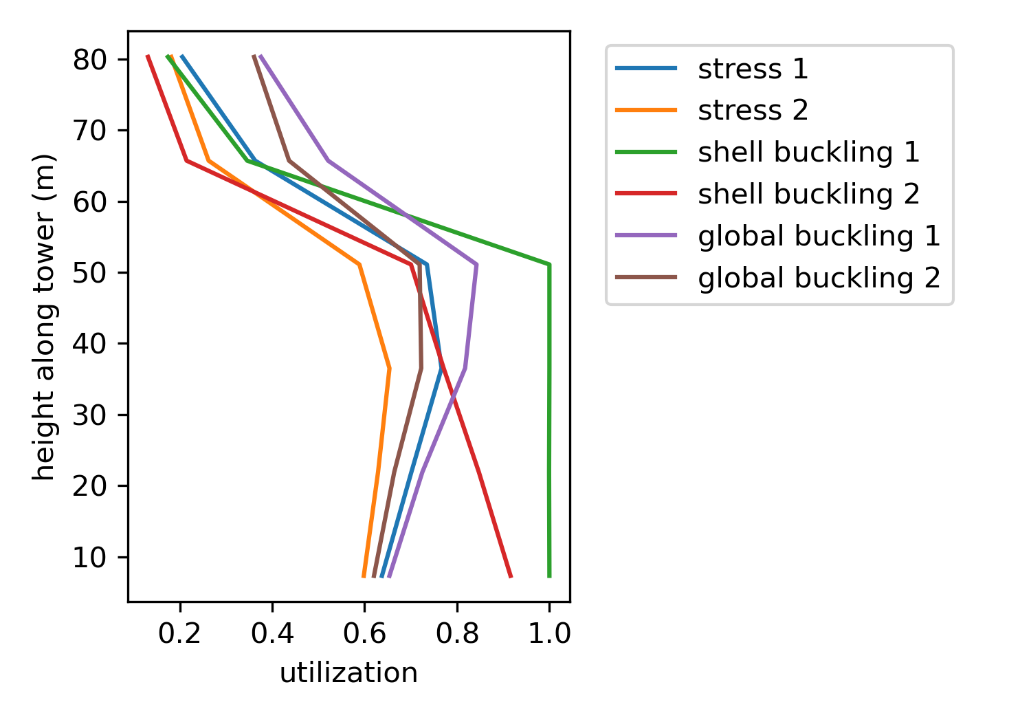
Fig. 10 Utilization along tower for ultimate stress, shell buckling, global buckling, and fatigue damage.
Offshore Monopile Design
Monopile design in WISDEM is modeled as an extension of the tower. In this example, the tower from above is applied offshore with the key differences being:
Tower base is now at 10m above the water level at a transition piece coupling with the monopile
Monopile extends from 10m above the water level through to the sea floor, at a water depth of 30m, with the pile extending an additional 25m into the surface.
Monopile also has three sections, with one section for the submerged pile, the middle section for the water column, and the top section above the water up until the transition piece.
Maximum allowable diameter for the monopile is 8m
Invoking with YAML files
To run just the monopile, there is an additional monopile section that must be added to the components section of the yaml,
    monopile:
        transition_piece_mass: 100e3
        transition_piece_cost: 100e3
        outer_shape_bem:
            reference_axis: &ref_axis_mono
                x:
                    grid: [0.0, 1.0]
                    values: [0.0, 0.0]
                y:
                    grid: [0.0, 1.0]
                    values: [0.0, 0.0]
                z:
                    grid: &grid_mono [0., 0.3846, 0.8462, 1.0]
                    values: [-55.0, -30.0, 0.0, 10.0]
            outer_diameter:
                grid: *grid_mono
                values: [8.0, 8.0, 8.0, 8.0]
            drag_coefficient:
                grid: [0.0, 1.0]
                values: [1.0, 1.0]
        internal_structure_2d_fem:
            outfitting_factor: 1.07
            reference_axis: *ref_axis_mono
            layers:
                - name: tower_wall
                  material: steel
                  thickness:
                    grid: *grid_mono
                    values: [0.055, 0.055, 0.055, 0.055]
The environment section must also be updated with the offshore properties,
    shear_exp: 0.1
    water_density: 1025.0
    water_dyn_viscosity: 1.3351e-3
    water_depth: 30.0
    significant_wave_height: 4.52
    significant_wave_period: 9.45
    soil_shear_modulus: 140.e+6
    soil_poisson: 0.4
The modeling_options_monopile.yaml file already contains a section for the monopile, with entries identical to the tower section. The input loading scenarios are also the same. The analysis_options.yaml file, however, is different and activates the design variables and constraints associated with the monopile. Note also that the objective function now says structural_mass, to capture the combined mass of both the tower and monopile,
general:
        folder_output: outputs
        fname_output: refturb_output
design_variables:

    tower:
        outer_diameter:
            flag: True
            lower_bound: 3.87
            upper_bound: 8.0
        layer_thickness:
            flag: True
            lower_bound: 4e-3
            upper_bound: 2e-1
    monopile:
        outer_diameter:
            flag: True
            lower_bound: 3.87
            upper_bound: 8.0
        layer_thickness:
            flag: True
            lower_bound: 4e-3
            upper_bound: 2e-1

merit_figure: structural_mass

constraints:
    tower:
        height_constraint:
            flag: False
            lower_bound: 1.e-2
            upper_bound: 1.e-2
        stress:
            flag: True
        global_buckling:
            flag: True
        shell_buckling:
            flag: True
        d_to_t:
            flag: False
            lower_bound: 120.0
            upper_bound: 2000.0
        taper:
            flag: False
            lower_bound: 0.2
        slope:
            flag: True
        frequency_1:
            flag: False
            lower_bound: 0.13
            upper_bound: 0.40
    monopile:
        stress:
            flag: True
        global_buckling:
            flag: True
        shell_buckling:
            flag: True
        d_to_t:
            flag: False
            lower_bound: 120.0
            upper_bound: 2000.0
        taper:
            flag: False
            lower_bound: 0.2
        slope:
            flag: True
        thickness_slope:
            flag: True
        frequency_1:
            flag: True
            lower_bound: 0.13
            upper_bound: 0.20
        pile_depth:
            flag: True
            lower_bound: 0.0
        tower_diameter_coupling:
            flag: True

driver:
    optimization:
        flag: True            # Flag to enable optimization
        tol: 1.e-3            # Optimality tolerance
        max_major_iter: 10    # Maximum number of major design iterations (SNOPT)
        max_minor_iter: 100   # Maximum number of minor design iterations (SNOPT)
        max_iter: 1         # Maximum number of iterations (SLSQP)
        solver: SLSQP         # Optimization solver. Other options are 'SLSQP' - 'CONMIN'
        step_size: 1.e-3      # Step size for finite differencing
        form: forward         # Finite differencing mode, either forward or central
    design_of_experiments:
        flag: False           # Flag to enable design of experiments
        run_parallel: True    # Flag to run using parallel processing
        generator: Uniform    # Type of input generator. (Uniform)
        num_samples: 5        # number of samples for (Uniform only)

recorder:
    flag: False                            # Flag to activate OpenMDAO recorder
    file_name: log_opt.sql    # Name of OpenMDAO recorder
The yaml files can be called directly from the command line, or via a python script that passes them to the top-level WISDEM function,
$ wisdem nrel5mw_monopile.yaml modeling_options_monopile.yaml analysis_options_monopile.yaml
or
$ python monopile_driver.py
Where the contents of monopile_driver.py are,
import os

from wisdem import run_wisdem

## File management
mydir = os.path.dirname(os.path.realpath(__file__))  # get path to this file
fname_wt_input = mydir + os.sep + "nrel5mw_monopile.yaml"
fname_modeling_options = mydir + os.sep + "modeling_options_monopile.yaml"
fname_analysis_options = mydir + os.sep + "analysis_options_monopile.yaml"

wt_opt, analysis_options, opt_options = run_wisdem(fname_wt_input, fname_modeling_options, fname_analysis_options)
Calling Python Directly
The monopile optimization script using direct calls to WISDEM’s TowerSE module also resembles the tower code, with some key additions to expand the design accordingly. First, the script setup now includes the monopile initial condition and the transition piece location between the monopile and tower. In this script, \(z=0\) corresponds to the mean sea level (MSL).
# Optimization by flag
# Two load cases
import os

import numpy as np
import openmdao.api as om

from wisdem.commonse.fileIO import save_data
from wisdem.fixed_bottomse.monopile import MonopileSE

# Set analysis and optimization options and define geometry
plot_flag = False
opt_flag = True

n_control_points = 4
n_materials = 1
n_load_cases = 2
max_diam = 8.0

# Tower initial condition
hubH = 87.6
htrans = 10.0

# Monopile initial condition
pile_depth = 25.0
water_depth = 30.0
h_paramM = np.r_[pile_depth, water_depth, htrans]
d_paramM = 0.9 * max_diam * np.ones(n_control_points)
t_paramM = 0.02 * np.ones(n_control_points)
The modeling options only needs to add in the number of sections and control points for the monopile,
modeling_options = {}
modeling_options["flags"] = {}
modeling_options["materials"] = {}
modeling_options["materials"]["n_mat"] = n_materials
modeling_options["WISDEM"] = {}
modeling_options["WISDEM"]["n_dlc"] = n_load_cases
modeling_options["WISDEM"]["FixedBottomSE"] = {}
modeling_options["WISDEM"]["FixedBottomSE"]["buckling_length"] = 15.0
modeling_options["WISDEM"]["FixedBottomSE"]["buckling_method"] = "dnvgl"
modeling_options["WISDEM"]["FixedBottomSE"]["n_refine"] = 3
modeling_options["flags"]["monopile"] = True
modeling_options["flags"]["tower"] = False

# Monopile foundation
modeling_options["WISDEM"]["FixedBottomSE"]["soil_springs"] = True
modeling_options["WISDEM"]["FixedBottomSE"]["gravity_foundation"] = False

# safety factors
modeling_options["WISDEM"]["FixedBottomSE"]["gamma_f"] = 1.35
modeling_options["WISDEM"]["FixedBottomSE"]["gamma_m"] = 1.3
modeling_options["WISDEM"]["FixedBottomSE"]["gamma_n"] = 1.0
modeling_options["WISDEM"]["FixedBottomSE"]["gamma_b"] = 1.1
modeling_options["WISDEM"]["FixedBottomSE"]["gamma_fatigue"] = 1.35 * 1.3 * 1.0

# Frame3DD options
modeling_options["WISDEM"]["FixedBottomSE"]["frame3dd"] = {}
modeling_options["WISDEM"]["FixedBottomSE"]["frame3dd"]["shear"] = True
modeling_options["WISDEM"]["FixedBottomSE"]["frame3dd"]["geom"] = True
modeling_options["WISDEM"]["FixedBottomSE"]["frame3dd"]["tol"] = 1e-7
modeling_options["WISDEM"]["FixedBottomSE"]["frame3dd"]["modal_method"] = 1

modeling_options["WISDEM"]["FixedBottomSE"]["n_height"] = n_control_points
modeling_options["WISDEM"]["FixedBottomSE"]["n_layers"] = 1
modeling_options["WISDEM"]["FixedBottomSE"]["wind"] = "PowerWind"
Next, we instantiate the OpenMDAO problem as before,
prob = om.Problem(reports=False)
prob.model = MonopileSE(modeling_options=modeling_options)
The optimization problem switches the objective function to the total structural mass of the tower plus the monopile, and the monopile diameter and thickness schedule are appended to the list of design variables.
if opt_flag:
    # Choose the optimizer to use
    prob.driver = om.ScipyOptimizeDriver()
    prob.driver.options["optimizer"] = "SLSQP"
    prob.driver.options["maxiter"] = 40

    # Add objective
    # prob.model.add_objective('tower_mass', ref=1e6) # Only tower
    # prob.model.add_objective("structural_mass", ref=1e6)  # Both
    prob.model.add_objective("monopile_mass", ref=1e6)  # Only monopile

    # Add design variables, in this case the tower diameter and wall thicknesses
    prob.model.add_design_var("monopile_outer_diameter_in", lower=3.87, upper=max_diam)
    prob.model.add_design_var("monopile_layer_thickness", lower=4e-3, upper=2e-1, ref=1e-2)

    # Add constraints on the tower design
    prob.model.add_constraint("post.constr_stress", upper=1.0)
    prob.model.add_constraint("post.constr_global_buckling", upper=1.0)
    prob.model.add_constraint("post.constr_shell_buckling", upper=1.0)
    prob.model.add_constraint("constr_d_to_t", lower=80.0, upper=500.0, ref=1e2)
    prob.model.add_constraint("constr_taper", lower=0.2)
    prob.model.add_constraint("slope", upper=1.0)
    prob.model.add_constraint("suctionpile_depth", lower=0.0)
    prob.model.add_constraint("f1", lower=0.13, upper=0.40, ref=0.1)
We then call setup() as before,
prob.setup()
Next, the additional inputs for the monopile include its discretization of the monopile and starting depth.
prob["water_depth"] = water_depth

prob["transition_piece_mass"] = 100e3

prob["monopile_foundation_height"] = -55.0
prob["tower_foundation_height"] = 10.0
prob["monopile_height"] = h_paramM.sum()
prob["monopile_s"] = np.cumsum(np.r_[0.0, h_paramM]) / h_paramM.sum()
prob["monopile_outer_diameter_in"] = d_paramM
prob["monopile_layer_thickness"] = t_paramM.reshape((1, -1))
prob["outfitting_factor_in"] = 1.07

prob["yaw"] = 0.0

# offshore specific
prob["G_soil"] = 140e6
prob["nu_soil"] = 0.4

# material properties
prob["E_mat"] = 210e9 * np.ones((n_materials, 3))
prob["G_mat"] = 79.3e9 * np.ones((n_materials, 3))
prob["rho_mat"] = [7850.0]
prob["sigma_y_mat"] = [345e6]
prob["sigma_ult_mat"] = 1.12e9 * np.ones((n_materials, 3))
prob["wohler_exp_mat"] = [4.0]
prob["wohler_A_mat"] = [4.0]

# cost rates
prob["unit_cost_mat"] = [2.0]  # USD/kg
prob["labor_cost_rate"] = 100.0 / 60.0  # USD/min
prob["painting_cost_rate"] = 30.0  # USD/m^2

# wind & wave values
prob["wind_reference_height"] = 90.0
prob["z0"] = 0.0
prob["cd_usr"] = -1.0
prob["rho_air"] = 1.225
prob["rho_water"] = 1025.0
prob["mu_air"] = 1.7934e-5
prob["mu_water"] = 1.3351e-3
prob["beta_wind"] = 0.0
prob["Hsig_wave"] = 4.52
prob["Tsig_wave"] = 9.52
if modeling_options["WISDEM"]["FixedBottomSE"]["wind"] == "PowerWind":
    prob["shearExp"] = 0.1
The offshore environment parameters, such as significant wave heights and water density, much also bet set,
prob["unit_cost_mat"] = [2.0]  # USD/kg
prob["labor_cost_rate"] = 100.0 / 60.0  # USD/min
prob["painting_cost_rate"] = 30.0  # USD/m^2

# wind & wave values
prob["wind_reference_height"] = 90.0
prob["z0"] = 0.0
prob["cd_usr"] = -1.0
prob["rho_air"] = 1.225
prob["rho_water"] = 1025.0
prob["mu_air"] = 1.7934e-5
prob["mu_water"] = 1.3351e-3
prob["beta_wind"] = 0.0
prob["Hsig_wave"] = 4.52
prob["Tsig_wave"] = 9.52
if modeling_options["WISDEM"]["FixedBottomSE"]["wind"] == "PowerWind":
    prob["shearExp"] = 0.1
The load cases are exactly the same as in the tower-only design case,
prob["env1.Uref"] = 11.73732
prob["env2.Uref"] = 70.0
prob["monopile.turbine_F"] = np.c_[[1.28474420e06, 0.0, -1.05294614e07], [9.30198601e05, 0.0, -1.13508479e07]]
prob["monopile.turbine_M"] = np.c_[
    [4009825.86806202, 92078894.58132489, -346781.68192839], [-1704977.30124085, 65817554.0892837, 147301.97023764]
]
We can now run the model and display some of the outputs, such as in Figure 11.
prob.model.approx_totals()
if opt_flag:
    prob.run_driver()
else:
    prob.run_model()
os.makedirs("outputs", exist_ok=True)
save_data(os.path.join("outputs", "monopile_example"), prob)
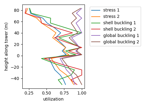
Fig. 11 Utilization along tower and monopile for ultimate stress, shell buckling, global buckling, and fatigue damage.